Solutions to Exercises from Mankiw's Book (Economics) | Microeconomics | Trường Đại học Quốc tế, Đại học Quốc gia Thành phố Hồ Chí Minh

SOLUTIONS TO TEXT PROBLEMS: Chapter 6 Quick Quizzes 1.
A price ceiling is a legal maximum on the price at which a good can be sold. Examples
of price ceilings include rent control, price controls on gasoline in the 1970s, and price
ceilings on water during a drought. A price floor is a legal minimum on the price at
which a good can be sold. Examples of price floors include the minimum wage and
farm-support prices. A price ceiling leads to a shortage, if the ceiling is binding, because
suppliers won’t produce enough goods to meet demand unless the price is allowed to rise
above the ceiling. A price floor leads to a surplus, if the floor is binding, because
suppliers produce more goods than are demanded unless the price is allowed to fall below the floor. 2.
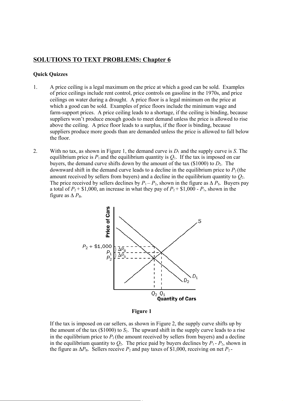
With no tax, as shown in Figure 1, the demand curve is D and the supply curve is 1 . The S
equilibrium price is P and the equilibrium quantity is 1
Q . If the tax is imposed on car 1
buyers, the demand curve shifts down by the amount of the tax ($1000) to D . The 2
downward shift in the demand curve leads to a decline in the equilibrium price to P (the 2
amount received by sellers from buyers) and a decline in the equilibrium quantity to Q2.
The price received by sellers declines by P1 – P2, shown in the figure as  PS. Buyers pay
a total of P + $1,000, an increase in what they pay of 2
P2 + $1,000 - P1, shown in the figure as  PB. Figure 1
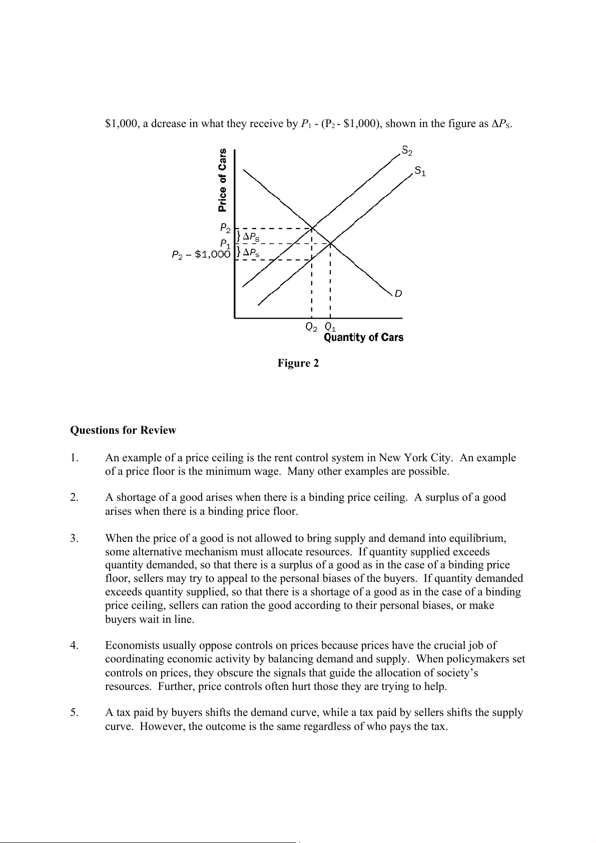
If the tax is imposed on car sellers, as shown in Figure 2, the supply curve shifts up by
the amount of the tax ($1000) to S . The upward shift in the supply curve leads to a rise 2
in the equilibrium price to P (the amount received by sellers from buyers) and a decline 2
in the equilibrium quantity to Q2. The price paid by buyers declines by P1 - P , shown in 2
the figure as PB. Sellers receive P and pay taxes of $1,000, receiving on net 2 P - 2
$1,000, a dcrease in what they receive by P1 - (P - $1,000), shown in the figure as 2 PS. Figure 2 Questions for Review 1.
An example of a price ceiling is the rent control system in New York City. An example
of a price floor is the minimum wage. Many other examples are possible. 2.
A shortage of a good arises when there is a binding price ceiling. A surplus of a good
arises when there is a binding price floor. 3.
When the price of a good is not allowed to bring supply and demand into equilibrium,
some alternative mechanism must allocate resources. If quantity supplied exceeds
quantity demanded, so that there is a surplus of a good as in the case of a binding price
floor, sellers may try to appeal to the personal biases of the buyers. If quantity demanded
exceeds quantity supplied, so that there is a shortage of a good as in the case of a binding
price ceiling, sellers can ration the good according to their personal biases, or make buyers wait in line. 4.
Economists usually oppose controls on prices because prices have the crucial job of
coordinating economic activity by balancing demand and supply. When policymakers set
controls on prices, they obscure the signals that guide the allocation of society’s
resources. Further, price controls often hurt those they are trying to help. 5.
A tax paid by buyers shifts the demand curve, while a tax paid by sellers shifts the supply
curve. However, the outcome is the same regardless of who pays the tax. 6.
A tax on a good raises the price buyers pay, lowers the price sellers receive, and reduces the quantity sold. 7.
The burden of a tax is divided between buyers and sellers depending on the elasticity of
demand and supply. Elasticity represents the willingness of buyers or sellers to leave the
market, which in turns depends on their alternatives. When a good is taxed, the side of
the market with fewer good alternatives cannot easily leave the market and thus bears more of the burden of the tax.
Problems and Applications 1.
If the price ceiling of $40 per ticket is below the equilibrium price, then quantity
demanded exceeds quantity supplied, so there will be a shortage of tickets. The policy
decreases the number of people who attend classical music concerts, since the quantity
supplied is lower because of the lower price. 2. a.
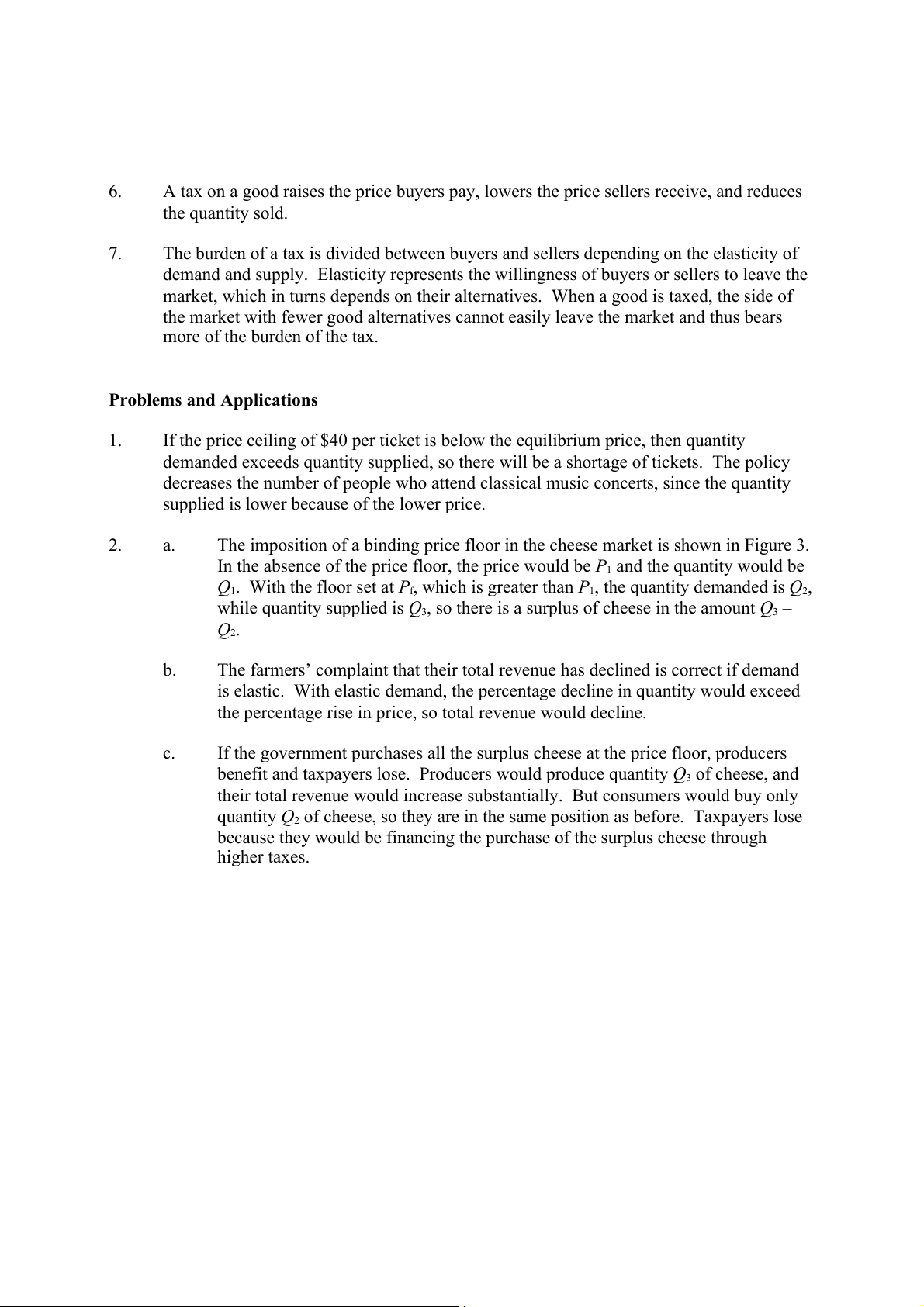
The imposition of a binding price floor in the cheese market is shown in Figure 3.
In the absence of the price floor, the price would be P and the quantity would be 1
Q1. With the floor set at Pf, which is greater than P1, the quantity demanded is Q , 2
while quantity supplied is Q , so there is a surplus of cheese in the amount 3 Q – 3 Q2. b.
The farmers’ complaint that their total revenue has declined is correct if demand
is elastic. With elastic demand, the percentage decline in quantity would exceed
the percentage rise in price, so total revenue would decline. c.
If the government purchases all the surplus cheese at the price floor, producers
benefit and taxpayers lose. Producers would produce quantity Q of cheese, and 3
their total revenue would increase substantially. But consumers would buy only
quantity Q2 of cheese, so they are in the same position as before. Taxpayers lose
because they would be financing the purchase of the surplus cheese through higher taxes. Figure 3 3. a.
The equilibrium price of Frisbees is $8 and the equilibrium quantity is 6 million Frisbees. b.
With a price floor of $10, the new market price is $10 since the price floor is
binding. At that price, only 2 million Frisbees are sold, since that’s the quantity demanded. c.
If there’s a price ceiling of $9, it has no effect, since the market equilibrium price
is $8, below the ceiling. So the equilibrium price is $8 and the equilibrium
quantity is 6 million Frisbees. 4. a.
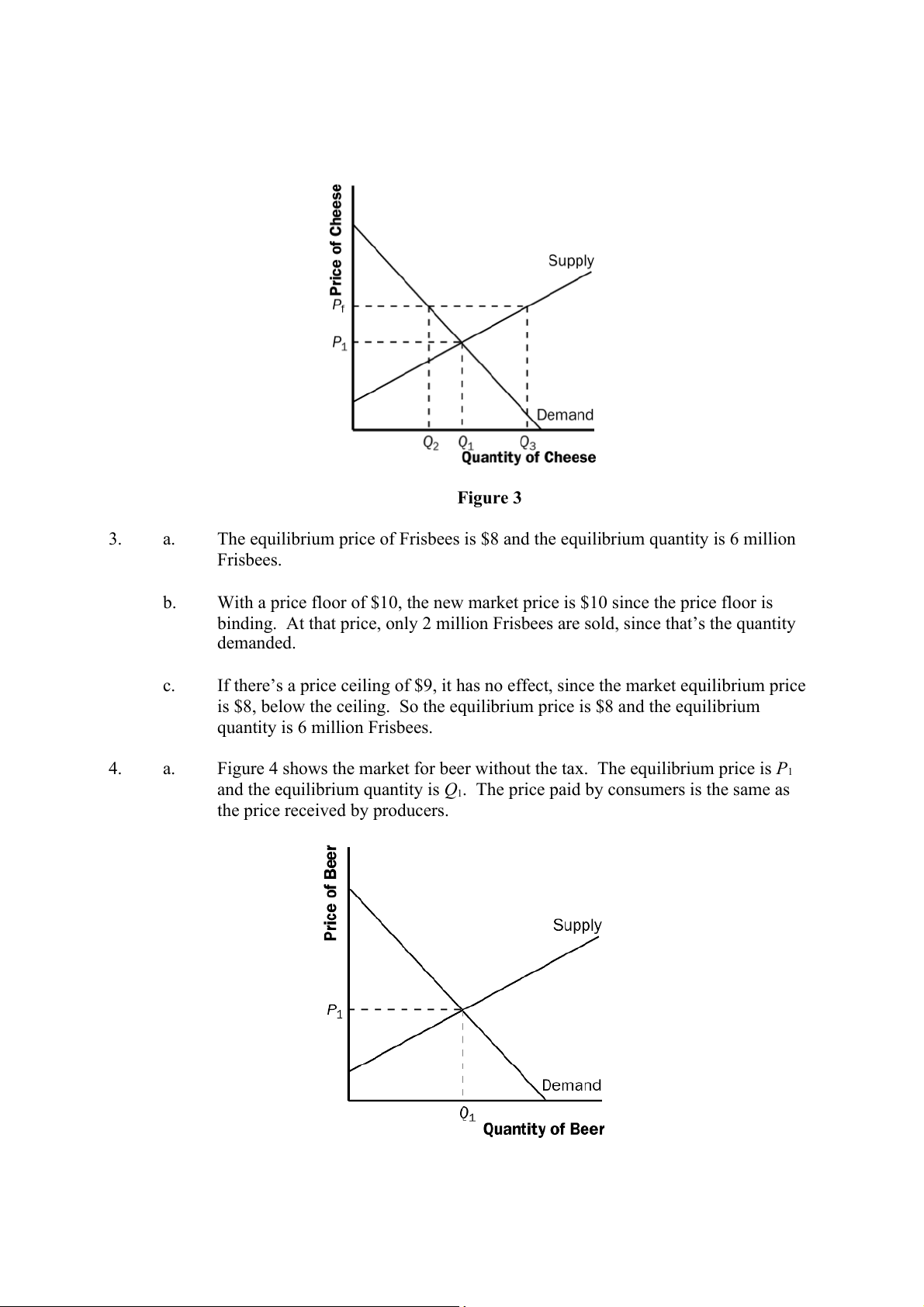
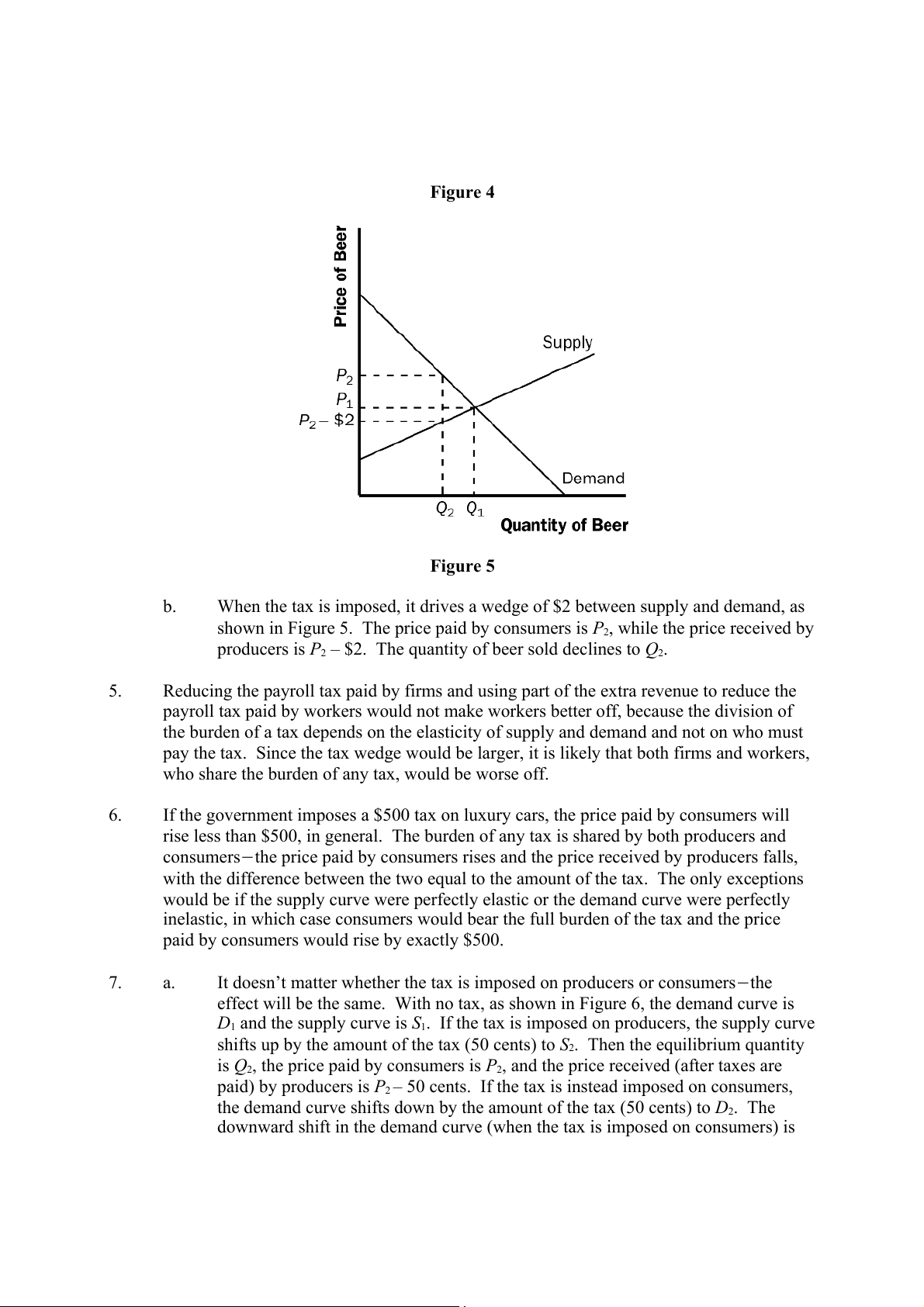
Figure 4 shows the market for beer without the tax. The equilibrium price is P1
and the equilibrium quantity is Q . The price paid by consumers is the same as 1
the price received by producers. Figure 4 Figure 5 b.
When the tax is imposed, it drives a wedge of $2 between supply and demand, as
shown in Figure 5. The price paid by consumers is P , while the price received by 2
producers is P – $2. The quantity of beer sold declines to 2 Q . 2 5.
Reducing the payroll tax paid by firms and using part of the extra revenue to reduce the
payroll tax paid by workers would not make workers better off, because the division of
the burden of a tax depends on the elasticity of supply and demand and not on who must
pay the tax. Since the tax wedge would be larger, it is likely that both firms and workers,
who share the burden of any tax, would be worse off. 6.
If the government imposes a $500 tax on luxury cars, the price paid by consumers will
rise less than $500, in general. The burden of any tax is shared by both producers and
consumersthe price paid by consumers rises and the price received by producers falls,
with the difference between the two equal to the amount of the tax. The only exceptions
would be if the supply curve were perfectly elastic or the demand curve were perfectly
inelastic, in which case consumers would bear the full burden of the tax and the price
paid by consumers would rise by exactly $500. 7. a.
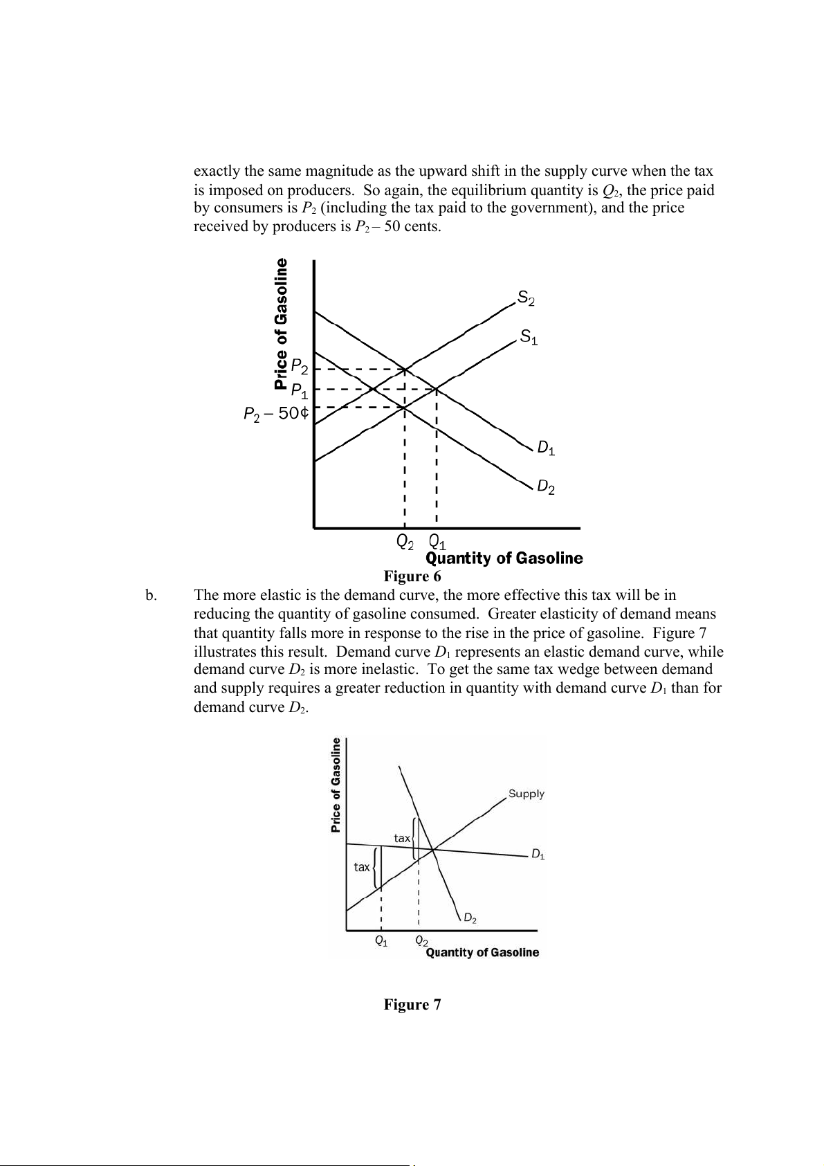
It doesn’t matter whether the tax is imposed on producers or consumersthe
effect will be the same. With no tax, as shown in Figure 6, the demand curve is
D1 and the supply curve is S . If the tax is imposed on producers, the supply curve 1
shifts up by the amount of the tax (50 cents) to S . Then the equilibrium quantity 2
is Q2, the price paid by consumers is P , and the price receive 2 d (after taxes are
paid) by producers is P2 – 50 cents. If the tax is instead imposed on consumers,
the demand curve shifts down by the amount of the tax (50 cents) to D . The 2
downward shift in the demand curve (when the tax is imposed on consumers) is
exactly the same magnitude as the upward shift in the supply curve when the tax
is imposed on producers. So again, the equilibrium quantity is Q2, the price paid
by consumers is P (including the tax paid to the government), and the price 2
received by producers is P – 50 cents. 2 Figure 6 b.
The more elastic is the demand curve, the more effective this tax will be in
reducing the quantity of gasoline consumed. Greater elasticity of demand means
that quantity falls more in response to the rise in the price of gasoline. Figure 7
illustrates this result. Demand curve D represents an elasti 1 c demand curve, while
demand curve D is more inelastic. To get the same tax wedge between demand 2
and supply requires a greater reduction in quantity with demand curve D than for 1 demand curve D . 2 Figure 7 c.
The consumers of gasoline are hurt by the tax because they get less gasoline at a higher price. d.
Workers in the oil industry are hurt by the tax as well. With a lower quantity of
gasoline being produced, some workers may lose their jobs. With a lower price
received by producers, wages of workers might decline. 8. a.
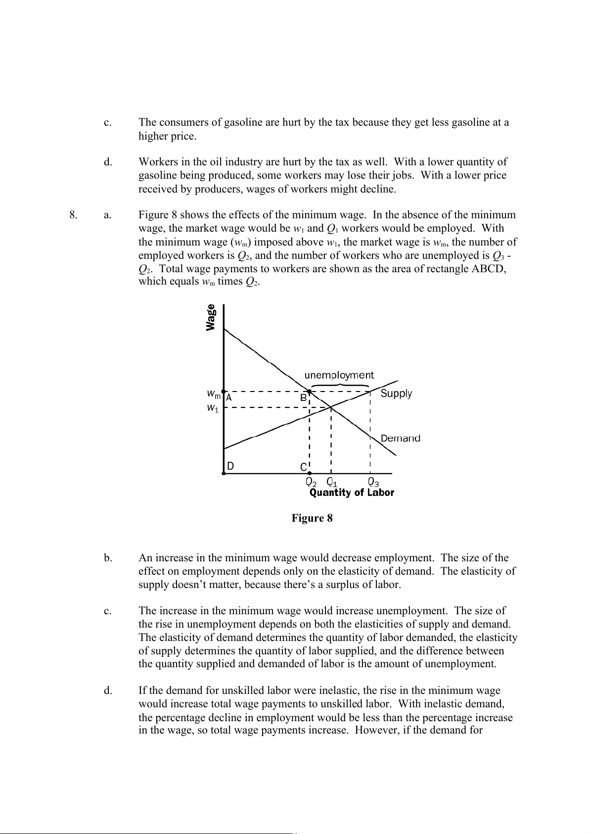
Figure 8 shows the effects of the minimum wage. In the absence of the minimum
wage, the market wage would be w and 1
Q workers would be employed. With 1
the minimum wage (wm) imposed above w1, the market wage is wm, the number of
employed workers is Q , and the number of workers who are unemployed is 2 Q - 3
Q2. Total wage payments to workers are shown as the area of rectangle ABCD,
which equals wm times Q . 2 Figure 8 b.
An increase in the minimum wage would decrease employment. The size of the
effect on employment depends only on the elasticity of demand. The elasticity of
supply doesn’t matter, because there’s a surplus of labor. c.
The increase in the minimum wage would increase unemployment. The size of
the rise in unemployment depends on both the elasticities of supply and demand.
The elasticity of demand determines the quantity of labor demanded, the elasticity
of supply determines the quantity of labor supplied, and the difference between
the quantity supplied and demanded of labor is the amount of unemployment. d.
If the demand for unskilled labor were inelastic, the rise in the minimum wage
would increase total wage payments to unskilled labor. With inelastic demand,
the percentage decline in employment would be less than the percentage increase
in the wage, so total wage payments increase. However, if the demand for
unskilled labor were elastic, total wage payments would decline, since then the
percentage decline in employment would exceed the percentage increase in the wage. 9. a.
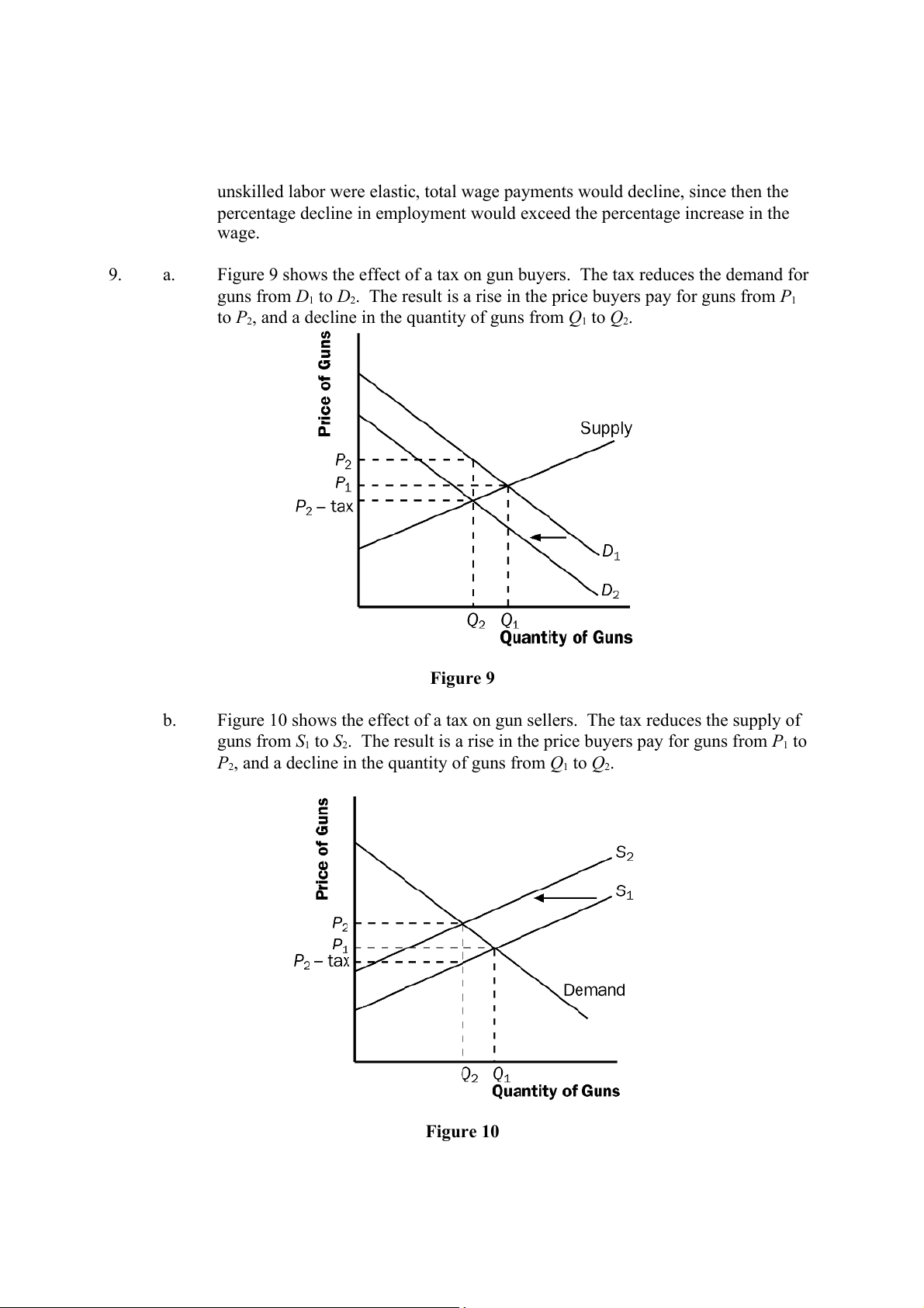
Figure 9 shows the effect of a tax on gun buyers. The tax reduces the demand for guns from D to 1
D . The result is a rise in the price buyers pay for guns from 2 P 1
to P2, and a decline in the quantity of guns from Q1 to Q2. Figure 9 b.
Figure 10 shows the effect of a tax on gun sellers. The tax reduces the supply of guns from S to 1
S2. The result is a rise in the price buyers pay for guns from P to 1
P2, and a decline in the quantity of guns from Q to 1 Q2. Figure 10 c.
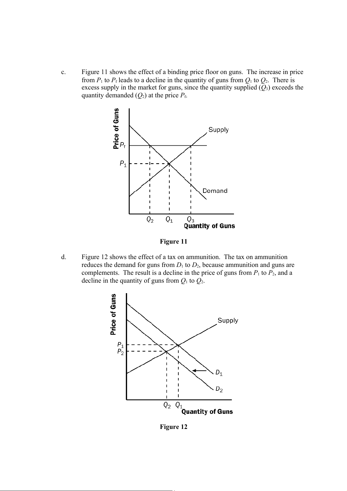
Figure 11 shows the effect of a binding price floor on guns. The increase in price
from P1 to Pf leads to a decline in the quantity of guns from Q to 1 Q2. There is
excess supply in the market for guns, since the quantity supplied (Q ) exceeds the 3
quantity demanded (Q ) at the price 2 Pf. Figure 11 d.
Figure 12 shows the effect of a tax on ammunition. The tax on ammunition
reduces the demand for guns from D to 1
D , because ammunition and guns are 2
complements. The result is a decline in the price of guns from P to 1 P2, and a
decline in the quantity of guns from Q to 1 Q . 2 Figure 12 10. a.
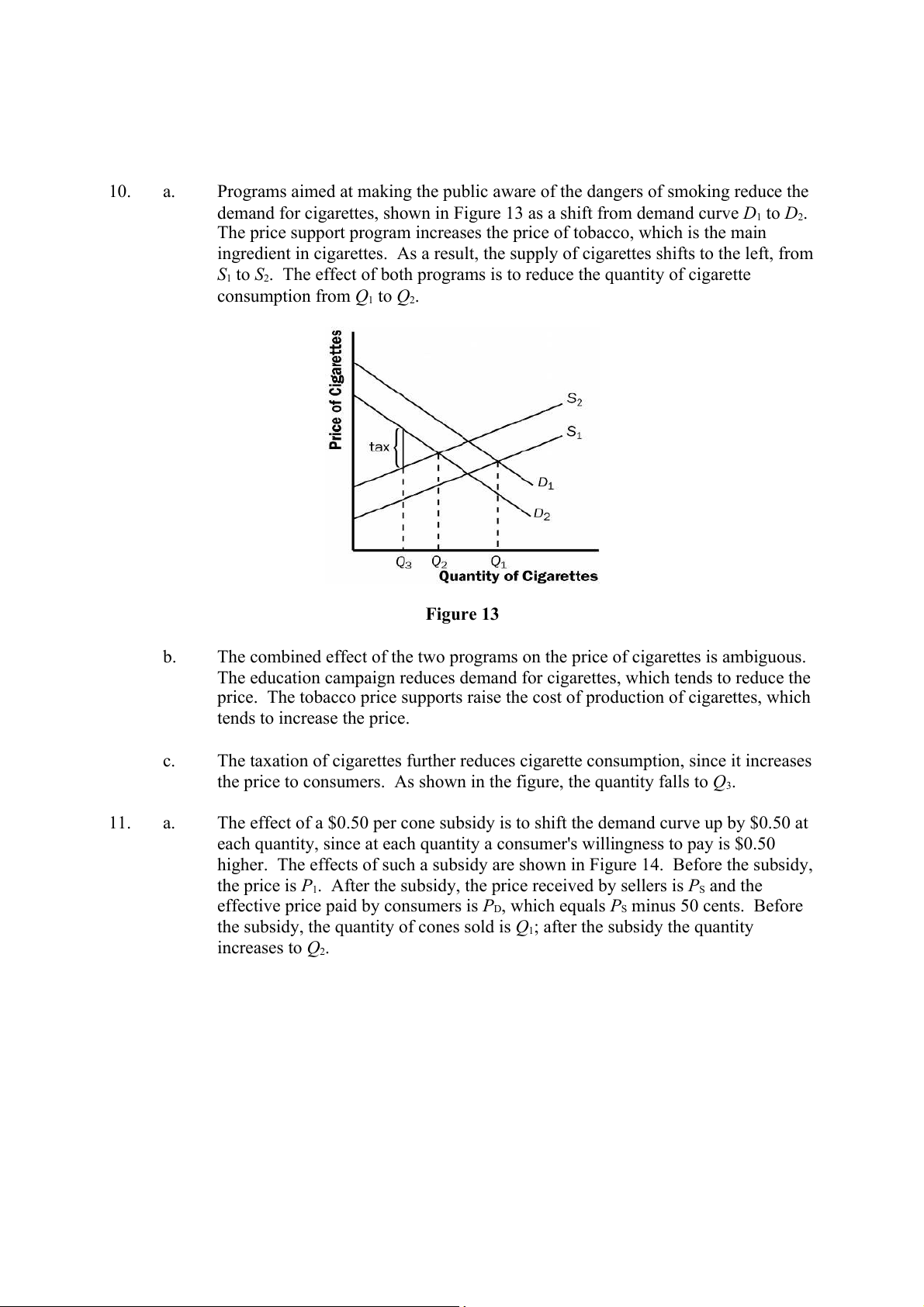
Programs aimed at making the public aware of the dangers of smoking reduce the
demand for cigarettes, shown in Figure 13 as a shift from demand curve D to 1 D . 2
The price support program increases the price of tobacco, which is the main
ingredient in cigarettes. As a result, the supply of cigarettes shifts to the left, from
S1 to S . The effect of both programs is to reduce the quantity of cigarette 2
consumption from Q1 to Q2. Figure 13 b.
The combined effect of the two programs on the price of cigarettes is ambiguous.
The education campaign reduces demand for cigarettes, which tends to reduce the
price. The tobacco price supports raise the cost of production of cigarettes, which tends to increase the price. c.
The taxation of cigarettes further reduces cigarette consumption, since it increases
the price to consumers. As shown in the figure, the quantity falls to Q . 3 11. a.
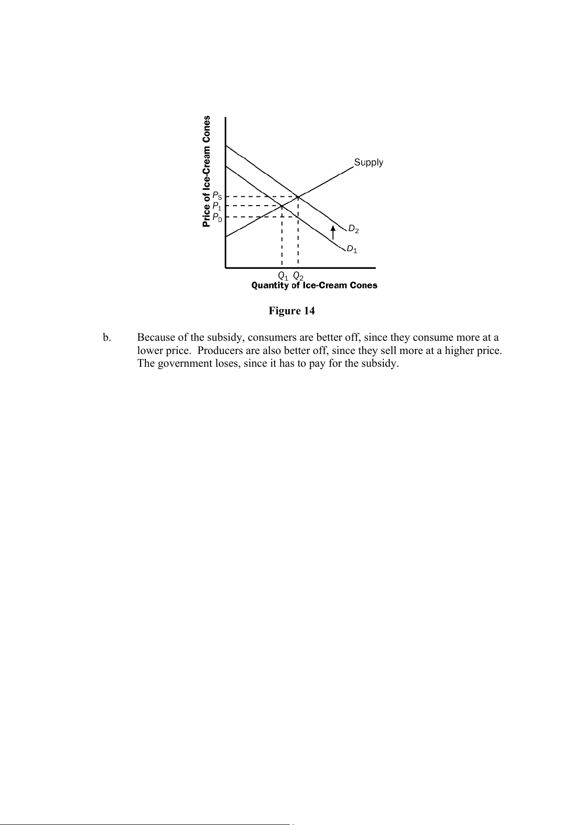
The effect of a $0.50 per cone subsidy is to shift the demand curve up by $0.50 at
each quantity, since at each quantity a consumer's willingness to pay is $0.50
higher. The effects of such a subsidy are shown in Figure 14. Before the subsidy,
the price is P . After the subsidy, the price received by sellers is 1 PS and the
effective price paid by consumers is PD, which equals PS minus 50 cents. Before
the subsidy, the quantity of cones sold is Q1; after the subsidy the quantity increases to Q . 2 Figure 14 b.
Because of the subsidy, consumers are better off, since they consume more at a
lower price. Producers are also better off, since they sell more at a higher price.
The government loses, since it has to pay for the subsidy.
SOLUTIONS TO TEXT PROBLEMS: Chapter 7 Quick Quizzes 1.
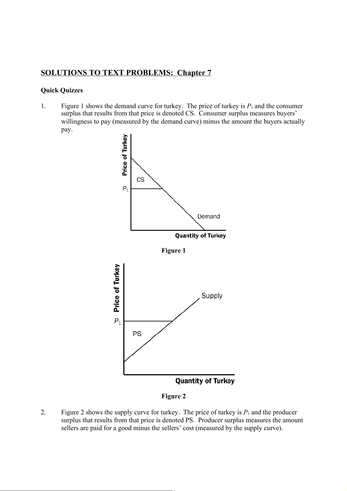
Figure 1 shows the demand curve for turkey. The price of turkey is P1 and the consumer
surplus that results from that price is denoted CS. Consumer surplus measures buyers’
willingness to pay (measured by the demand curve) minus the amount the buyers actually pay. Figure 1 Figure 2 2.
Figure 2 shows the supply curve for turkey. The price of turkey is P1 and the producer
surplus that results from that price is denoted PS. Producer surplus measures the amount
sellers are paid for a good minus the sellers’ cost (measured by the supply curve). Figure 3 3.
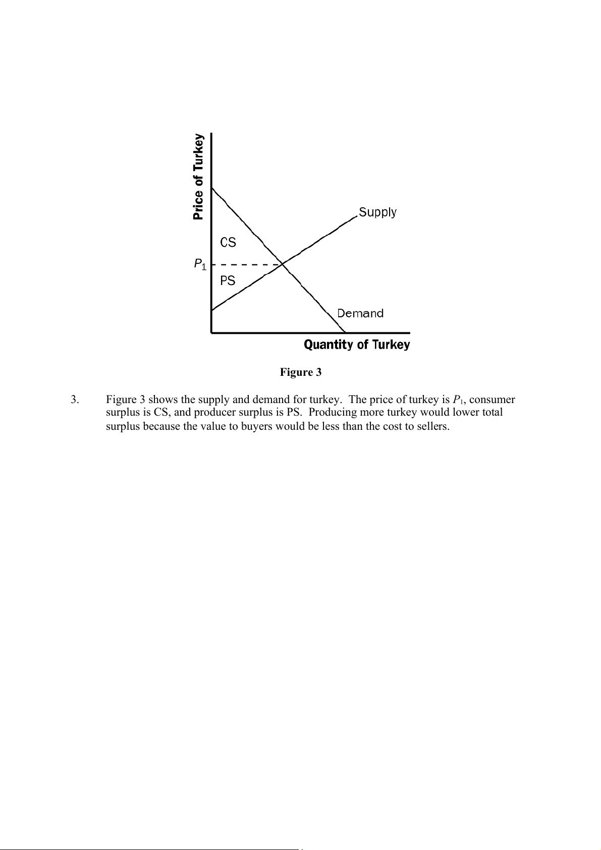
Figure 3 shows the supply and demand for turkey. The price of turkey is P1, consumer
surplus is CS, and producer surplus is PS. Producing more turkey would lower total
surplus because the value to buyers would be less than the cost to sellers. Questions for Review 1.
Buyers' willingness to pay, consumer surplus, and the demand curve are all closely
related. The height of the demand curve represents the willingness to pay of the buyers.
Consumer surplus is the area below the demand curve and above the price, which equals
each buyer's willingness to pay less the price of the good. 2.
Sellers' costs, producer surplus, and the supply curve are all closely related. The height
of the supply curve represents the costs of the sellers. Producer surplus is the area below
the price and above the supply curve, which equals the price minus each sellers' costs. Figure 4 3.
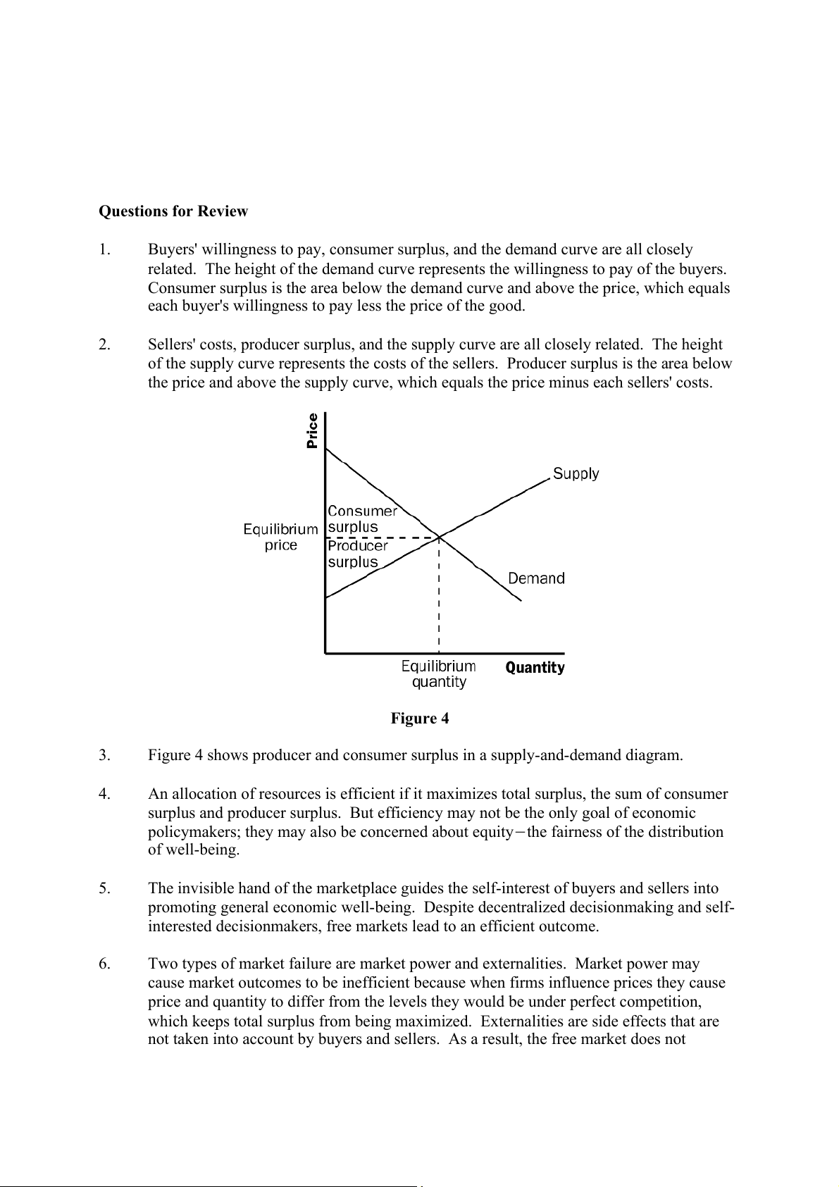
Figure 4 shows producer and consumer surplus in a supply-and-demand diagram. 4.
An allocation of resources is efficient if it maximizes total surplus, the sum of consumer
surplus and producer surplus. But efficiency may not be the only goal of economic
policymakers; they may also be concerned about equitythe fairness of the distribution of well-being. 5.
The invisible hand of the marketplace guides the self-interest of buyers and sellers into
promoting general economic well-being. Despite decentralized decisionmaking and self-
interested decisionmakers, free markets lead to an efficient outcome. 6.
Two types of market failure are market power and externalities. Market power may
cause market outcomes to be inefficient because when firms influence prices they cause
price and quantity to differ from the levels they would be under perfect competition,
which keeps total surplus from being maximized. Externalities are side effects that are
not taken into account by buyers and sellers. As a result, the free market does not maximize total surplus.
Problems and Applications 1.
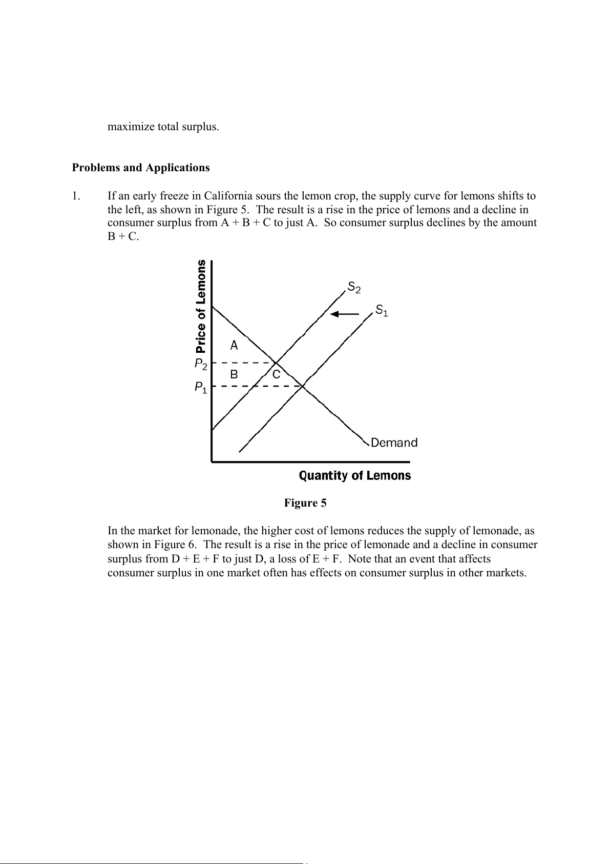
If an early freeze in California sours the lemon crop, the supply curve for lemons shifts to
the left, as shown in Figure 5. The result is a rise in the price of lemons and a decline in
consumer surplus from A + B + C to just A. So consumer surplus declines by the amount B + C. Figure 5
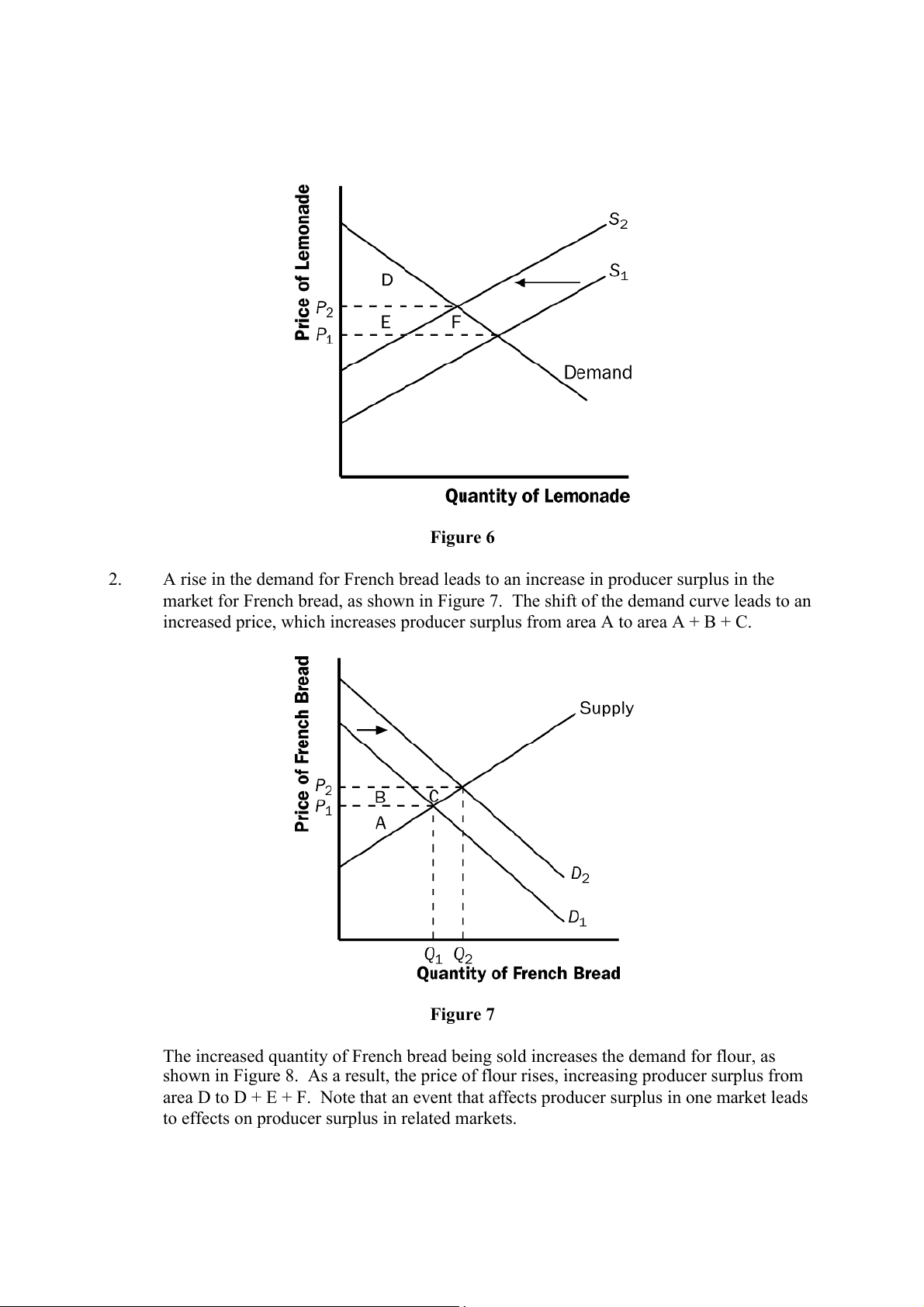
In the market for lemonade, the higher cost of lemons reduces the supply of lemonade, as
shown in Figure 6. The result is a rise in the price of lemonade and a decline in consumer
surplus from D + E + F to just D, a loss of E + F. Note that an event that affects
consumer surplus in one market often has effects on consumer surplus in other markets. Figure 6 2.
A rise in the demand for French bread leads to an increase in producer surplus in the
market for French bread, as shown in Figure 7. The shift of the demand curve leads to an
increased price, which increases producer surplus from area A to area A + B + C. Figure 7
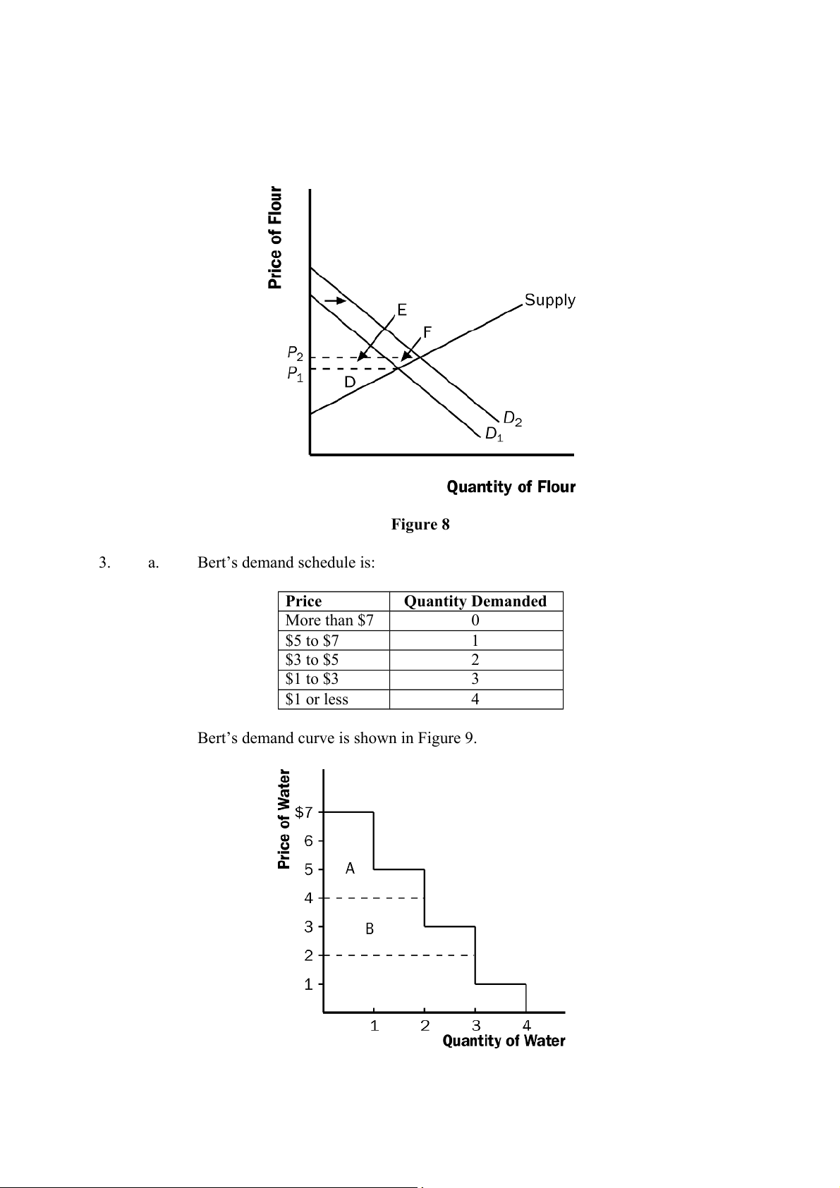
The increased quantity of French bread being sold increases the demand for flour, as
shown in Figure 8. As a result, the price of flour rises, increasing producer surplus from
area D to D + E + F. Note that an event that affects producer surplus in one market leads
to effects on producer surplus in related markets. Figure 8 3. a. Bert’s demand schedule is: Price Quantity Demanded More than $7 0 $5 to $7 1 $3 to $5 2 $1 to $3 3 $1 or less 4
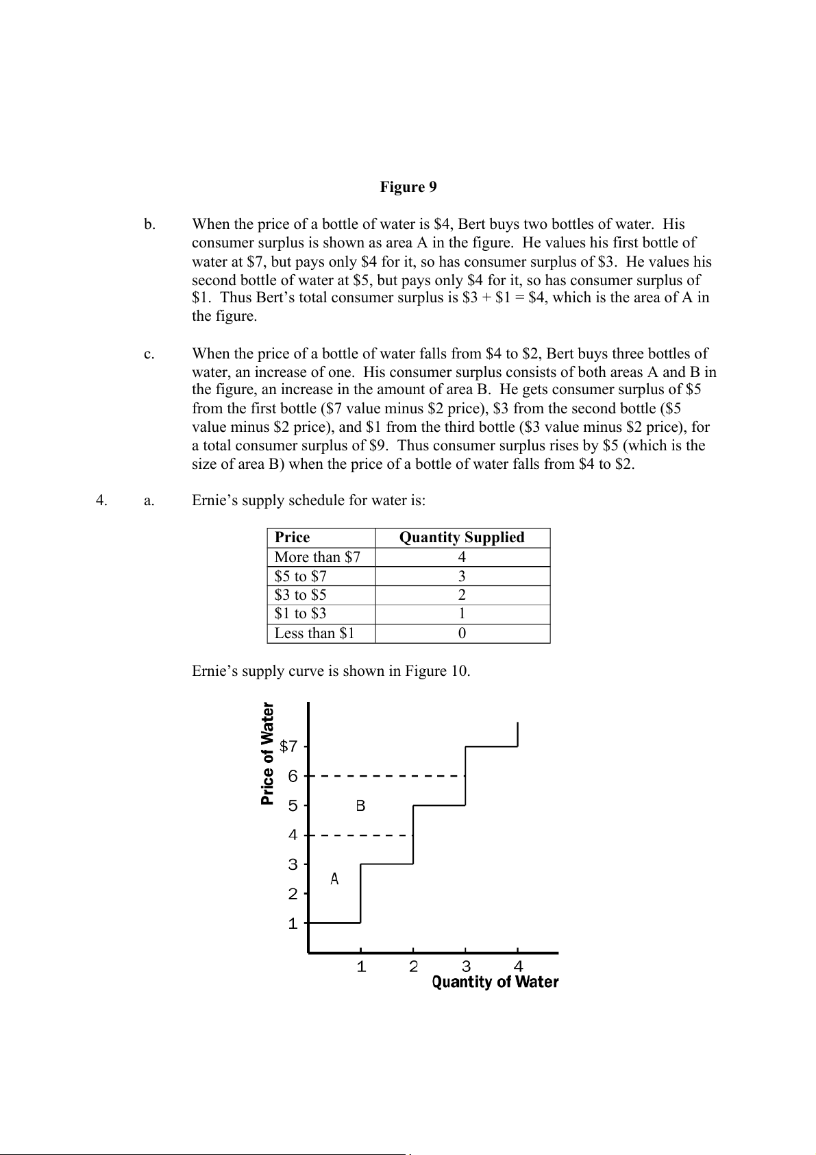
Bert’s demand curve is shown in Figure 9. Figure 9 b.
When the price of a bottle of water is $4, Bert buys two bottles of water. His
consumer surplus is shown as area A in the figure. He values his first bottle of
water at $7, but pays only $4 for it, so has consumer surplus of $3. He values his
second bottle of water at $5, but pays only $4 for it, so has consumer surplus of
$1. Thus Bert’s total consumer surplus is $3 + $1 = $4, which is the area of A in the figure. c.
When the price of a bottle of water falls from $4 to $2, Bert buys three bottles of
water, an increase of one. His consumer surplus consists of both areas A and B in
the figure, an increase in the amount of area B. He gets consumer surplus of $5
from the first bottle ($7 value minus $2 price), $3 from the second bottle ($5
value minus $2 price), and $1 from the third bottle ($3 value minus $2 price), for
a total consumer surplus of $9. Thus consumer surplus rises by $5 (which is the
size of area B) when the price of a bottle of water falls from $4 to $2. 4. a.
Ernie’s supply schedule for water is: Price Quantity Supplied More than $7 4 $5 to $7 3 $3 to $5 2 $1 to $3 1 Less than $1 0
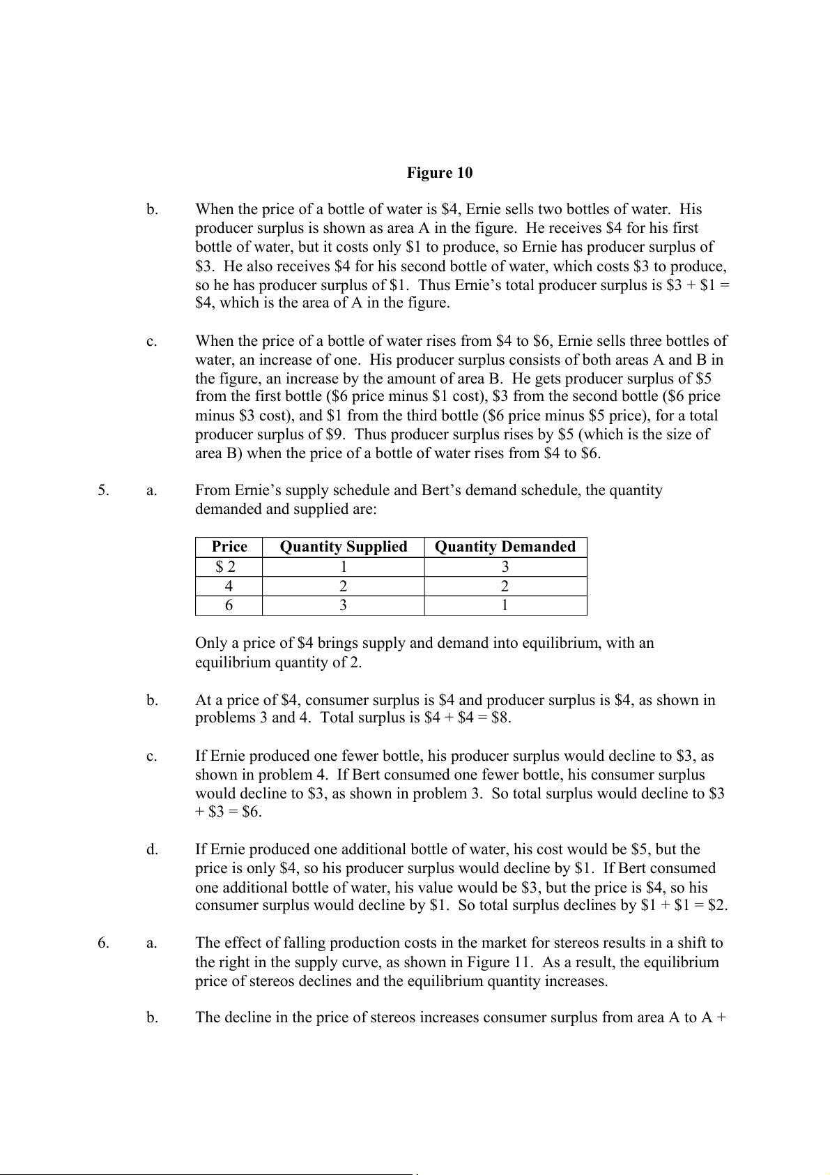
Ernie’s supply curve is shown in Figure 10. Figure 10 b.
When the price of a bottle of water is $4, Ernie sells two bottles of water. His
producer surplus is shown as area A in the figure. He receives $4 for his first
bottle of water, but it costs only $1 to produce, so Ernie has producer surplus of
$3. He also receives $4 for his second bottle of water, which costs $3 to produce,
so he has producer surplus of $1. Thus Ernie’s total producer surplus is $3 + $1 =
$4, which is the area of A in the figure. c.
When the price of a bottle of water rises from $4 to $6, Ernie sells three bottles of
water, an increase of one. His producer surplus consists of both areas A and B in
the figure, an increase by the amount of area B. He gets producer surplus of $5
from the first bottle ($6 price minus $1 cost), $3 from the second bottle ($6 price
minus $3 cost), and $1 from the third bottle ($6 price minus $5 price), for a total
producer surplus of $9. Thus producer surplus rises by $5 (which is the size of
area B) when the price of a bottle of water rises from $4 to $6. 5. a.
From Ernie’s supply schedule and Bert’s demand schedule, the quantity demanded and supplied are: Price Quantity Supplied Quantity Demanded $ 2 1 3 4 2 2 6 3 1
Only a price of $4 brings supply and demand into equilibrium, with an equilibrium quantity of 2. b.
At a price of $4, consumer surplus is $4 and producer surplus is $4, as shown in
problems 3 and 4. Total surplus is $4 + $4 = $8. c.
If Ernie produced one fewer bottle, his producer surplus would decline to $3, as
shown in problem 4. If Bert consumed one fewer bottle, his consumer surplus
would decline to $3, as shown in problem 3. So total surplus would decline to $3 + $3 = $6. d.
If Ernie produced one additional bottle of water, his cost would be $5, but the
price is only $4, so his producer surplus would decline by $1. If Bert consumed
one additional bottle of water, his value would be $3, but the price is $4, so his
consumer surplus would decline by $1. So total surplus declines by $1 + $1 = $2. 6. a.
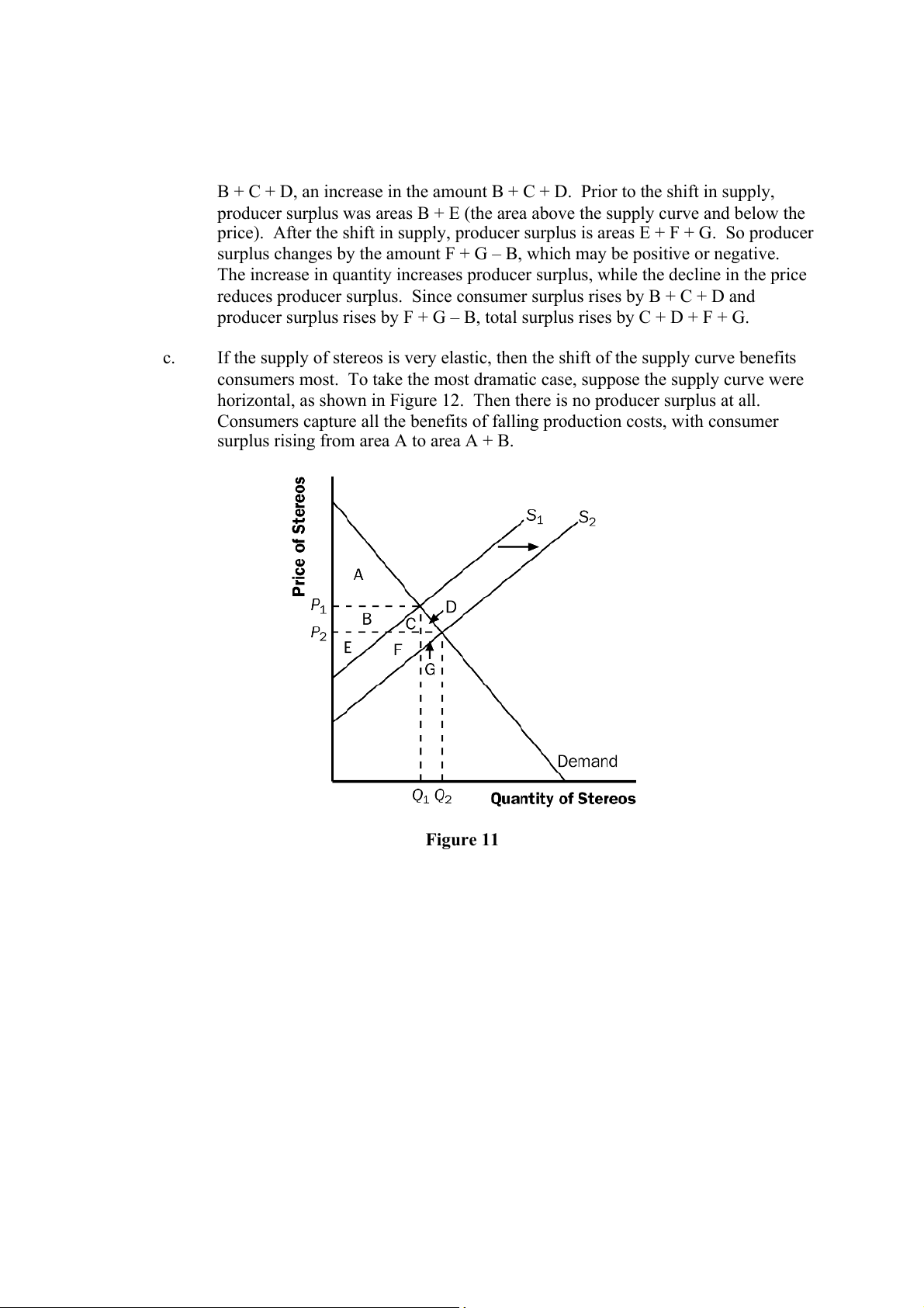
The effect of falling production costs in the market for stereos results in a shift to
the right in the supply curve, as shown in Figure 11. As a result, the equilibrium
price of stereos declines and the equilibrium quantity increases. b.
The decline in the price of stereos increases consumer surplus from area A to A +
B + C + D, an increase in the amount B + C + D. Prior to the shift in supply,
producer surplus was areas B + E (the area above the supply curve and below the
price). After the shift in supply, producer surplus is areas E + F + G. So producer
surplus changes by the amount F + G – B, which may be positive or negative.
The increase in quantity increases producer surplus, while the decline in the price
reduces producer surplus. Since consumer surplus rises by B + C + D and
producer surplus rises by F + G – B, total surplus rises by C + D + F + G. c.
If the supply of stereos is very elastic, then the shift of the supply curve benefits
consumers most. To take the most dramatic case, suppose the supply curve were
horizontal, as shown in Figure 12. Then there is no producer surplus at all.
Consumers capture all the benefits of falling production costs, with consumer
surplus rising from area A to area A + B. Figure 11