Understanding Supply and Demand Dynamics | Microeconomics | Trường Đại học Quốc tế, Đại học Quốc gia Thành phố Hồ Chí Minh
Buyers and Sellers in the Market • The market for any good consists of all the buyers and sellers of the good • Buyers and sellers have different motivations – Buyers want to benefit from the good – Sellers want to make a profit • Market price balances two forces – Value buyers derive from the good – Cost to produce the good. Tài liệu được sưu tầm và soạn thảo dưới dạng file PDF để gửi tới các bạn cùng tham khảo, ôn tập đầy đủ kiến thức, chuẩn bị cho các buổi học thật tốt. Mời bạn đọc đón xem!
Môn: Microeconomics 635 tài liệu
Trường: Trường Đại học Quốc tế, Đại học Quốc gia Thành phố Hồ Chí Minh 1.9 K tài liệu
Tác giả:

Preview text:
Chapter 3 Supply and Demand
© 2022 McGraw Hill. All rights reserved. Authorized only for instructor use in the classroom. No reproduction or distribution without the prior written consent of McGraw-Hill. Learning Objectives
1. Describe how the demand and supply curves summarize the behavior
of buyers and sellers in the marketplace.
2. Discuss how the supply and demand curves interact to determine
equilibrium price and quantity.
3. Illustrate how shifts in supply and demand curves cause prices and quantities to change
4. Explain and apply the Efficiency Principle and the Equilibrium
Principle (also called the ÒNo-Cash-on-the-Table PrincipleÓ). 2 © 2022 McGraw Hill. What, How, and for Whom?
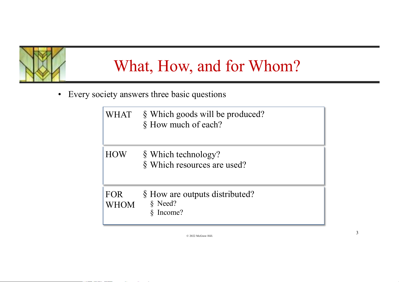
• Every society answers three basic questions WHAT
§ Which goods will be produced? § How much of each? HOW § Which technology? § Which resources are used? FOR
§ How are outputs distributed? WHOM § Need? § Income? 3 © 2022 McGraw Hill. Central Planning vs The Market Central Planning The Market
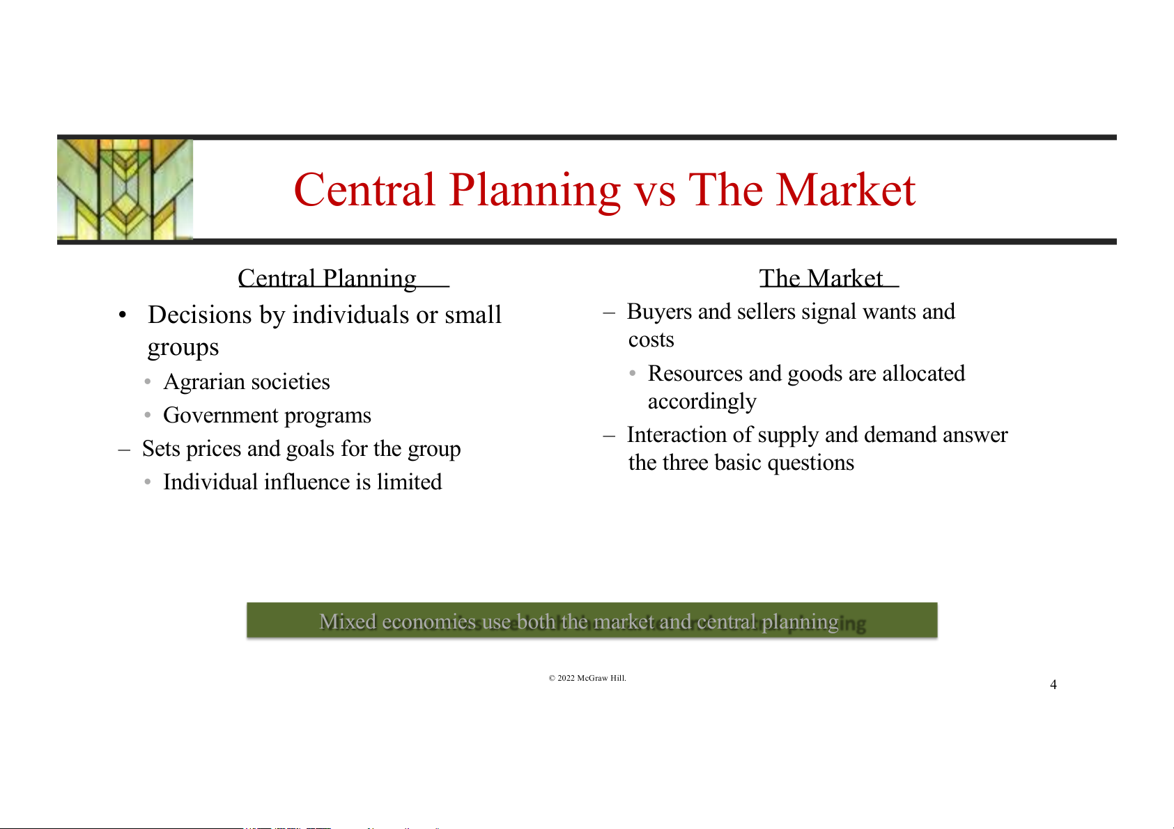
• Decisions by individuals or small
– Buyers and sellers signal wants and groups costs • Agrarian societies
• Resources and goods are allocated accordingly • Government programs
– Interaction of supply and demand answer
– Sets prices and goals for the group the three basic questions
• Individual influence is limited
Mixed economies use both the market and central planning © 2022 McGraw Hill. 4
Buyers and Sellers in the Market
• The market for any good consists of all the buyers and sellers of the good
• Buyers and sellers have different motivations
– Buyers want to benefit from the good
– Sellers want to make a profit
• Market price balances two forces
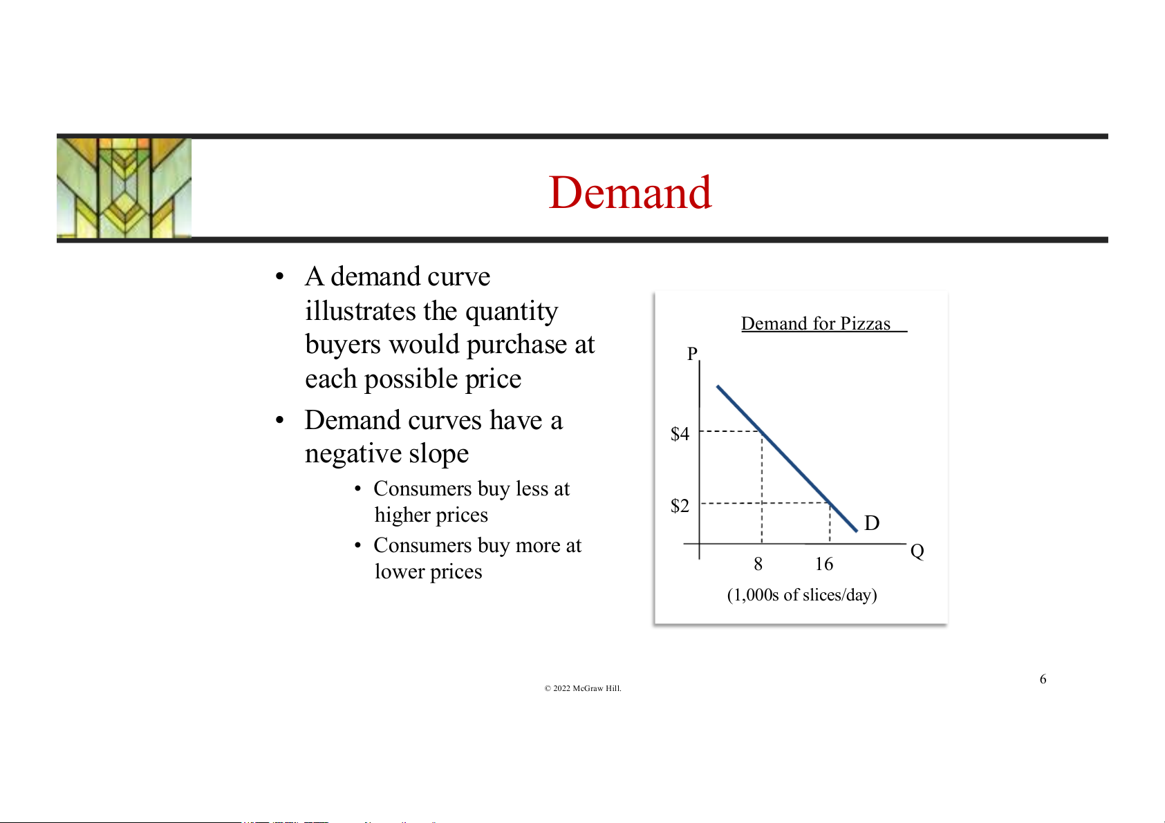
– Value buyers derive from the good – Cost to produce the good 5 © 2022 McGraw Hill. Demand • A demand curve illustrates the quantity Demand for Pizzas buyers would purchase at P each possible price • Demand curves have a $4 negative slope • Consumers buy less at higher prices $2 D • Consumers buy more at Q lower prices 8 16 (1,000s of slices/day) 6 © 2022 McGraw Hill. Demand Slopes Downward
• Buyers value goods differently
– The buyerÕs reservation price is the highest price an individual is willing to pay for a good
• Demand reflects the entire market, not one consumer
– Lower prices bring more buyers into the market
– Lower prices cause existing buyers to buy more 7 © 2022 McGraw Hill.
Income and Substitution Effects
• Buyers buy more at lower prices and buy less at higher prices
• What happens when price goes up?
– The substitution effect: Buyers switch to substitutes when price goes up
– The income effect: Buyers' overall purchasing power goes down 8 © 2022 McGraw Hill. Interpreting the Demand Curve • Horizontal interpretation Demand for Pizzas of demand: P
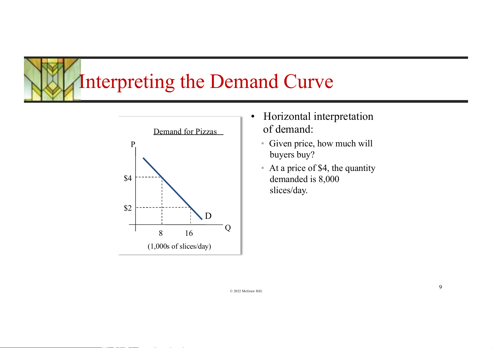
• Given price, how much will buyers buy?
• At a price of $4, the quantity $4 demanded is 8,000 slices/day. $2 D Q 8 16 (1,000s of slices/day) 9 © 2022 McGraw Hill. Interpreting the Demand Curve
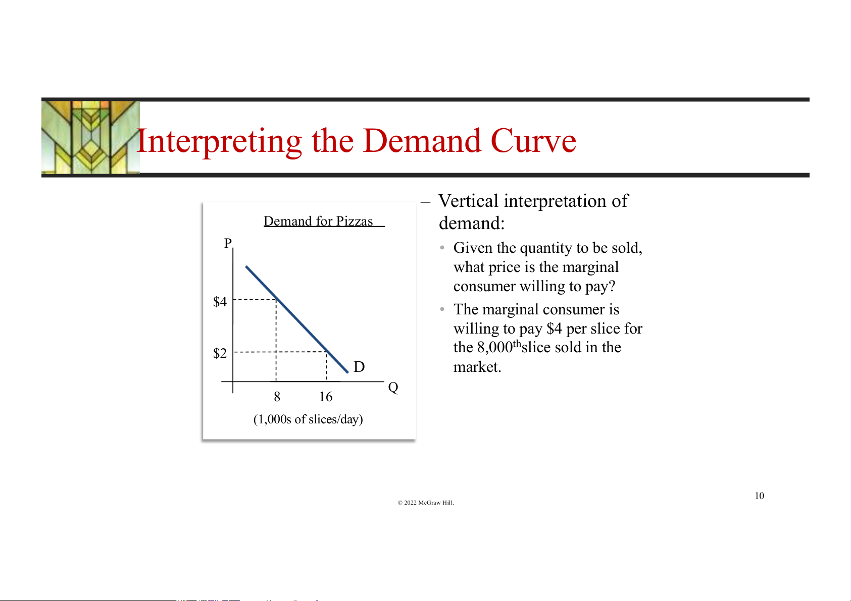
– Vertical interpretation of Demand for Pizzas demand: P
• Given the quantity to be sold, what price is the marginal consumer willing to pay? $4 • The marginal consumer is
willing to pay $4 per slice for the 8,000thslice sold in the $2 D market. Q 8 16 (1,000s of slices/day) 10 © 2022 McGraw Hill. The Supply Curve
• The supply curve illustrates the quantity of a good that sellers are willing to offer at each price
• Opportunity cost differs among sellers due to: § Technology
■ Different costs such as rent § Skills ■ Expectations
• The Low-Hanging Fruit Principle explains the upward sloping supply curve
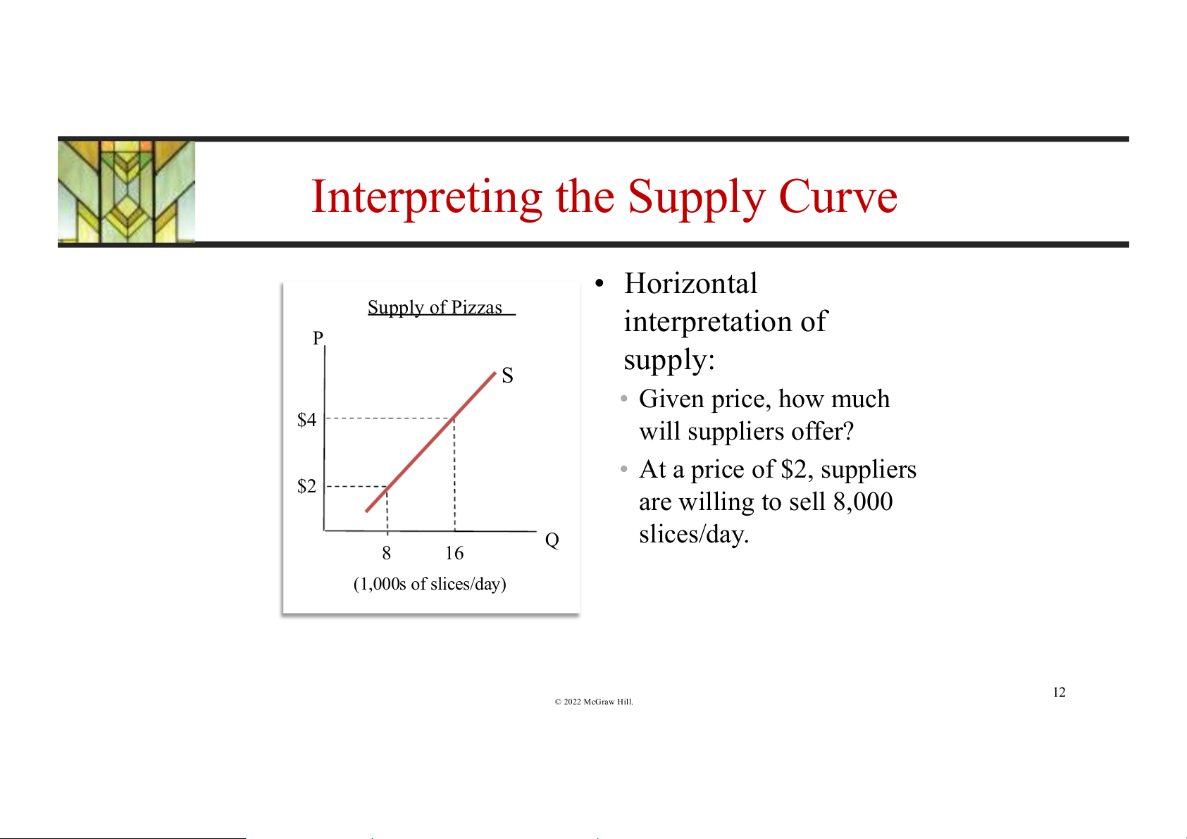
• The sellerÕs reservation price is the lowest price the seller would be willing to sell for – Equal to marginal cost 11 © 2022 McGraw Hill. Interpreting the Supply Curve • Horizontal Supply of Pizzas interpretation of P supply: S • Given price, how much $4 will suppliers offer?
• At a price of $2, suppliers $2 are willing to sell 8,000 Q slices/day. 8 16 (1,000s of slices/day) 12 © 2022 McGraw Hill. Interpreting the Supply Curve
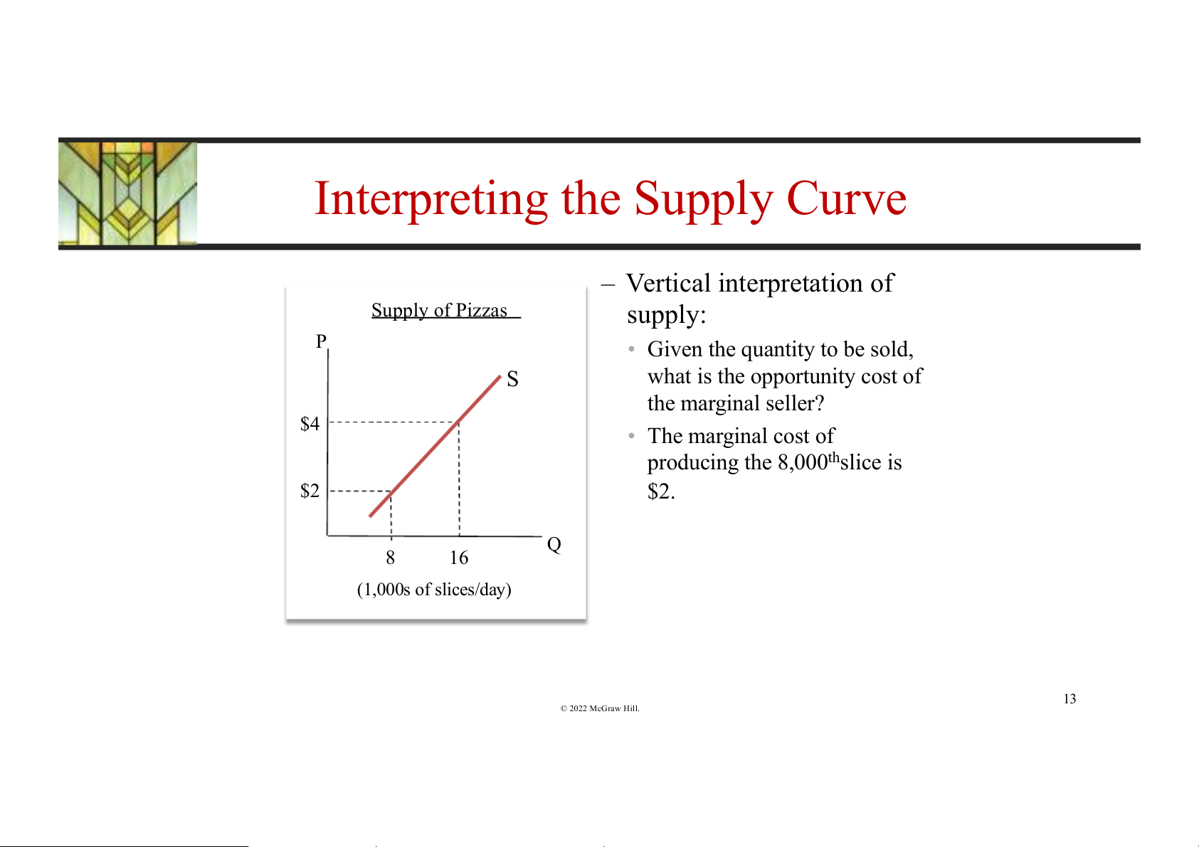
– Vertical interpretation of Supply of Pizzas supply: P
• Given the quantity to be sold, S
what is the opportunity cost of the marginal seller? $4 • The marginal cost of producing the 8,000thslice is $2 $2. Q 8 16 (1,000s of slices/day) 13 © 2022 McGraw Hill. Market Equilibrium
• A system is in equilibrium when there is no tendency for it to change
• The equilibrium price is the price at which the supply and demand curves intersect
• The equilibrium quantity is the quantity at which the supply and demand curves intersect
• The market equilibrium occurs when all buyers and sellers are satisfied
with their respective quantities at the market price
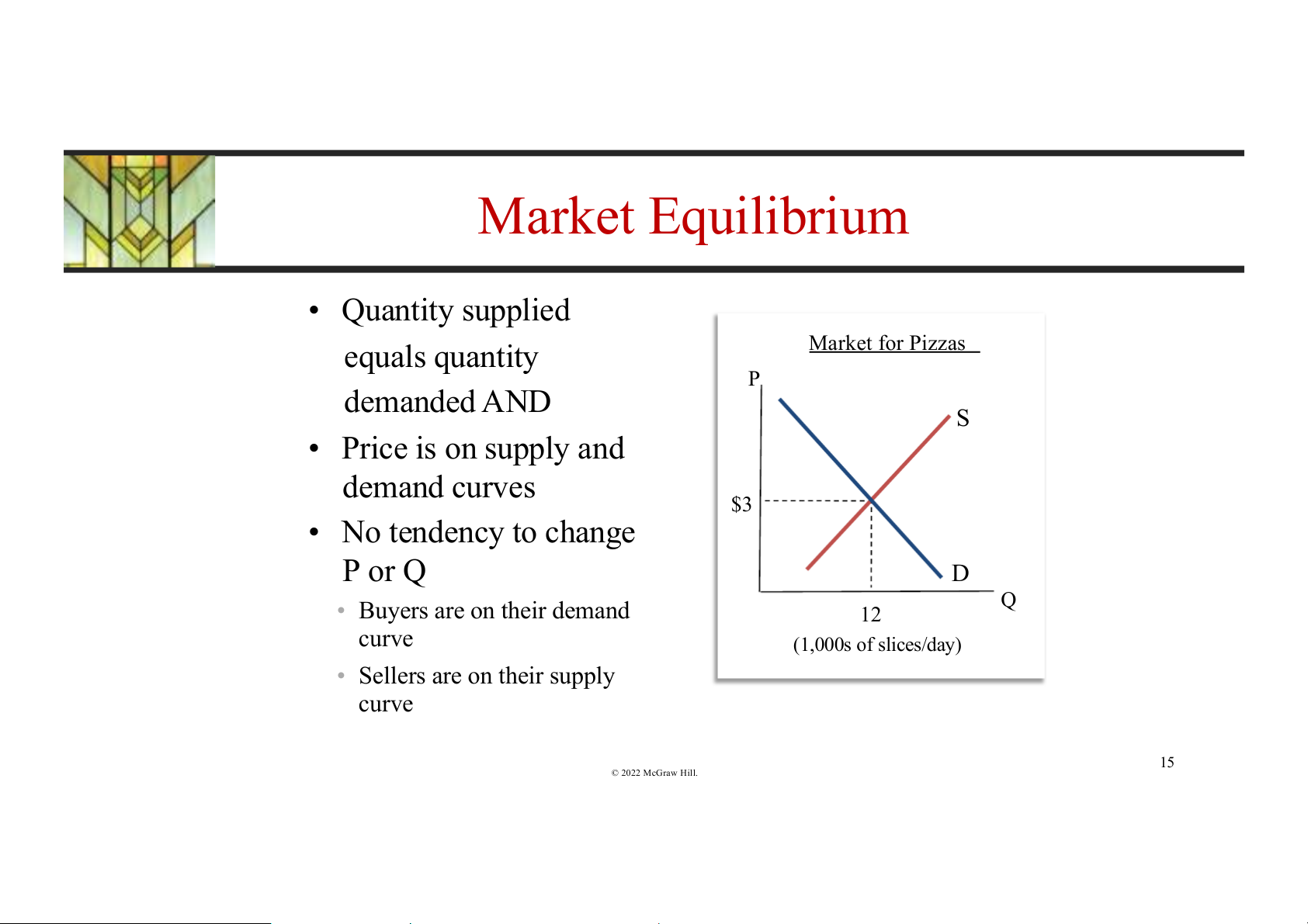
– At the equilibrium price, quantity supplied equals quantity demanded 14 © 2022 McGraw Hill. Market Equilibrium • Quantity supplied equals quantity Market for Pizzas P demanded AND S • Price is on supply and demand curves $3 • No tendency to change P or Q D
• Buyers are on their demand Q 12 curve (1,000s of slices/day)
• Sellers are on their supply curve 15 © 2022 McGraw Hill.
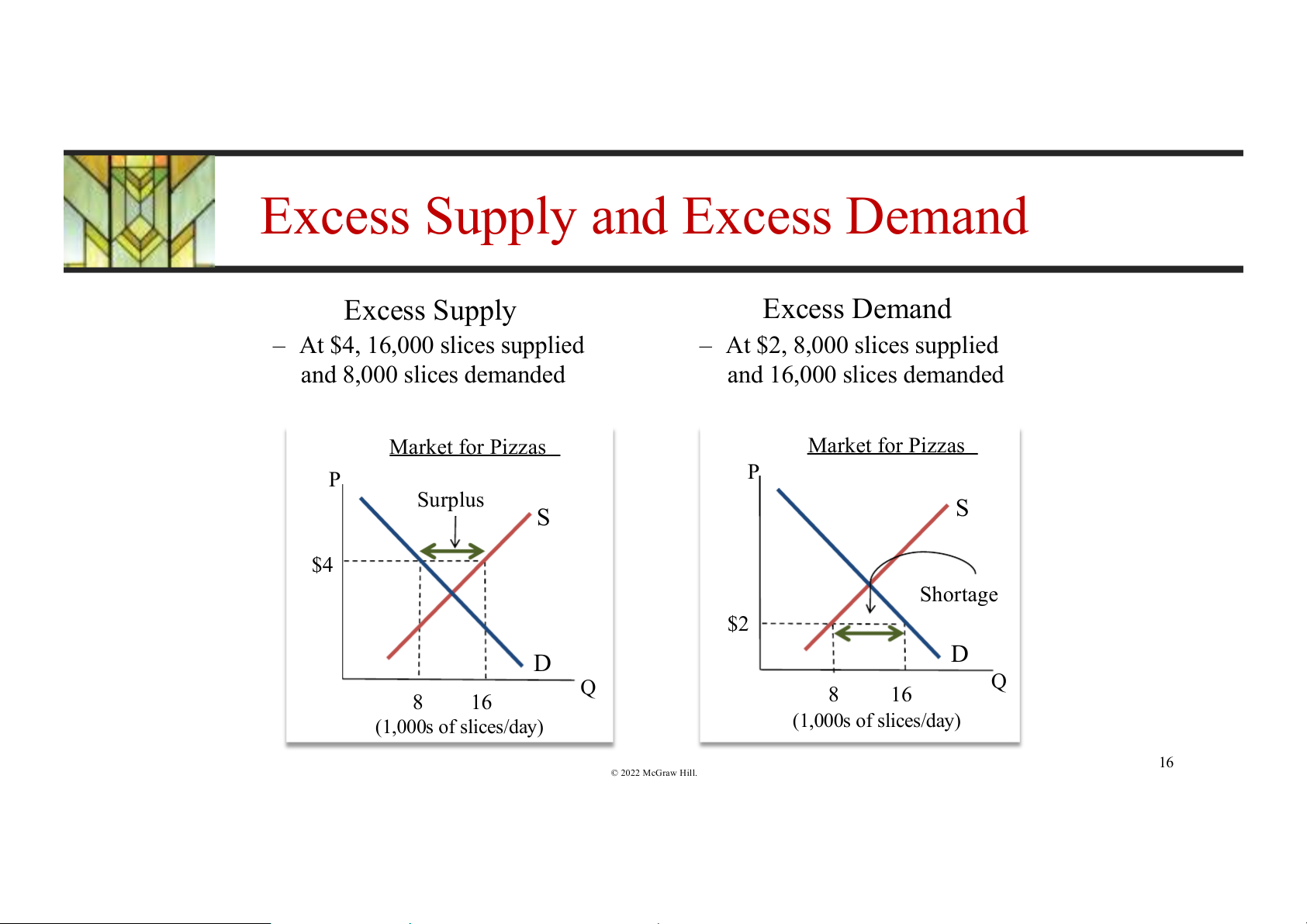
Excess Supply and Excess Demand Excess Supply Excess Demand
– At $4, 16,000 slices supplied
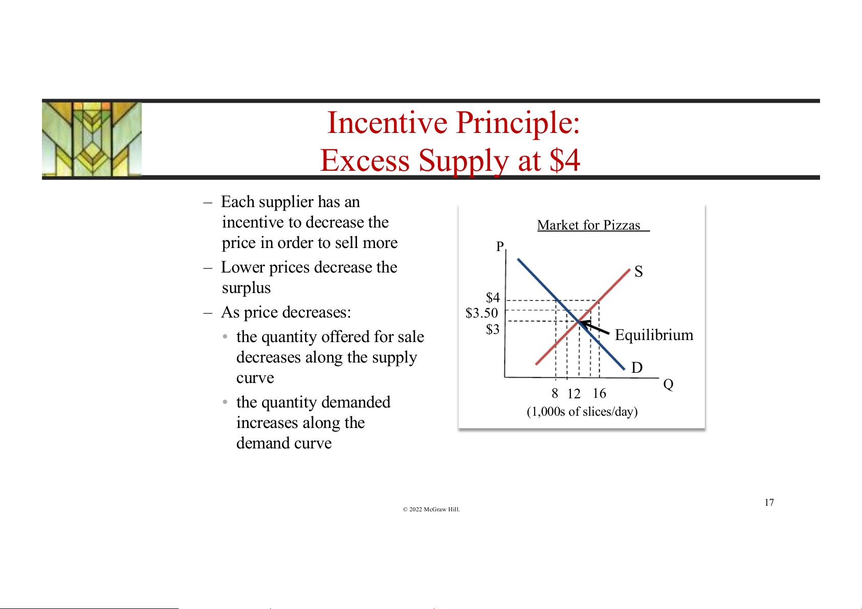
– At $2, 8,000 slices supplied and 8,000 slices demanded and 16,000 slices demanded Market for Pizzas Market for Pizzas P P Surplus S S $4 Shortage $2 D D Q Q 8 16 8 16 (1,000s of slices/day) (1,000s of slices/day) 16 © 2022 McGraw Hill. Incentive Principle: Excess Supply at $4 – Each supplier has an incentive to decrease the Market for Pizzas price in order to sell more P – Lower prices decrease the S surplus $4 – As price decreases: $3.50
• the quantity offered for sale $3 Equilibrium decreases along the supply curve D Q • the quantity demanded 8 12 16 (1,000s of slices/day) increases along the demand curve 17 © 2022 McGraw Hill. Incentive Principle: Excess Demand at $2 – Each supplier has an incentive to increase the Market for Pizzas price in order to sell more P
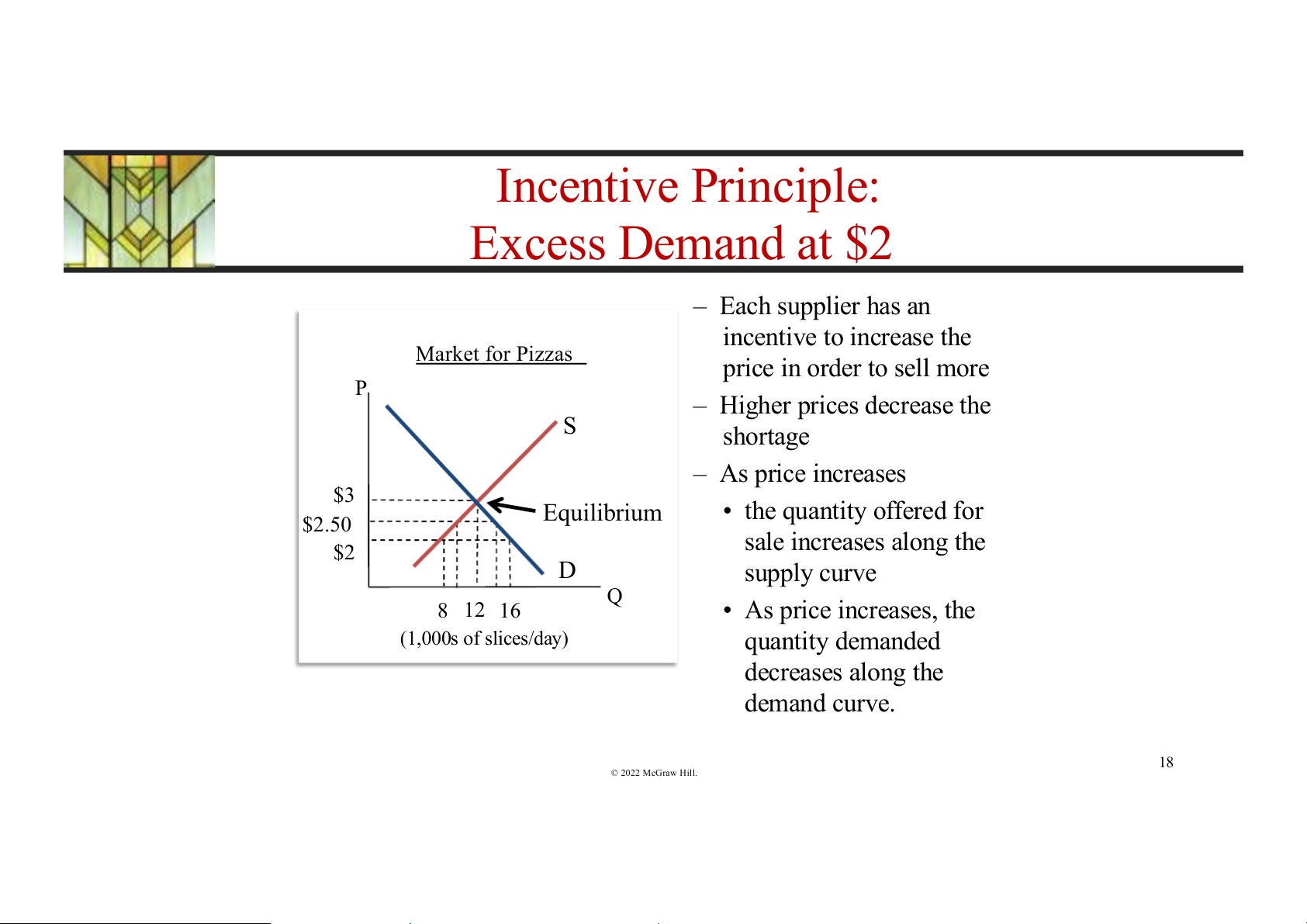
– Higher prices decrease the S shortage – As price increases $3 Equilibrium • the quantity offered for $2.50 sale increases along the $2 D supply curve Q 8 12 16 • As price increases, the (1,000s of slices/day) quantity demanded decreases along the demand curve. 18 © 2022 McGraw Hill.
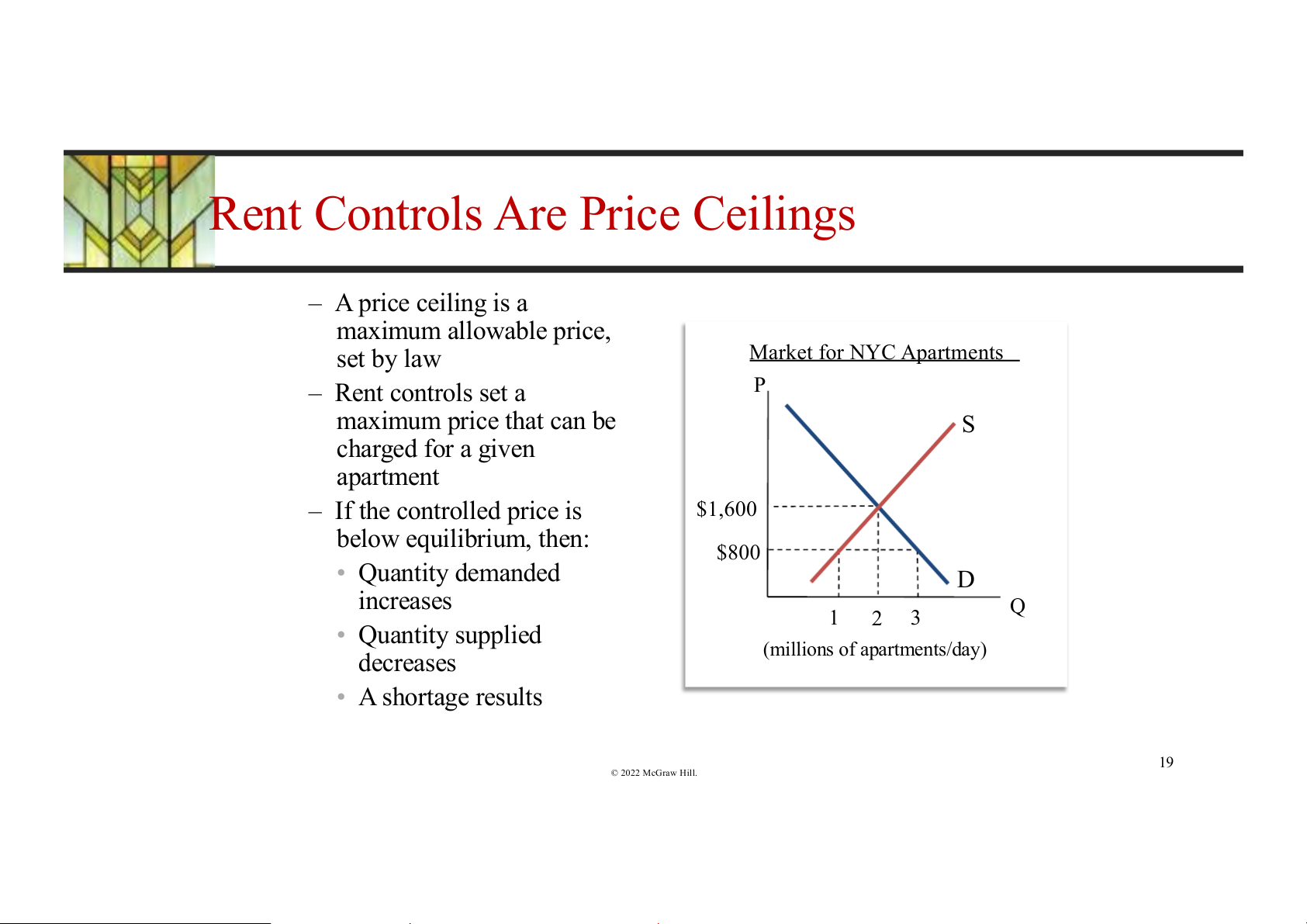
Rent Controls Are Price Ceilings – A price ceiling is a maximum allowable price, set by law Market for NYC Apartments – Rent controls set a P maximum price that can be S charged for a given apartment
– If the controlled price is $1,600 below equilibrium, then: $800 • Quantity demanded D increases Q 1 2 3 • Quantity supplied decreases (millions of apartments/day) • A shortage results 19 © 2022 McGraw Hill.
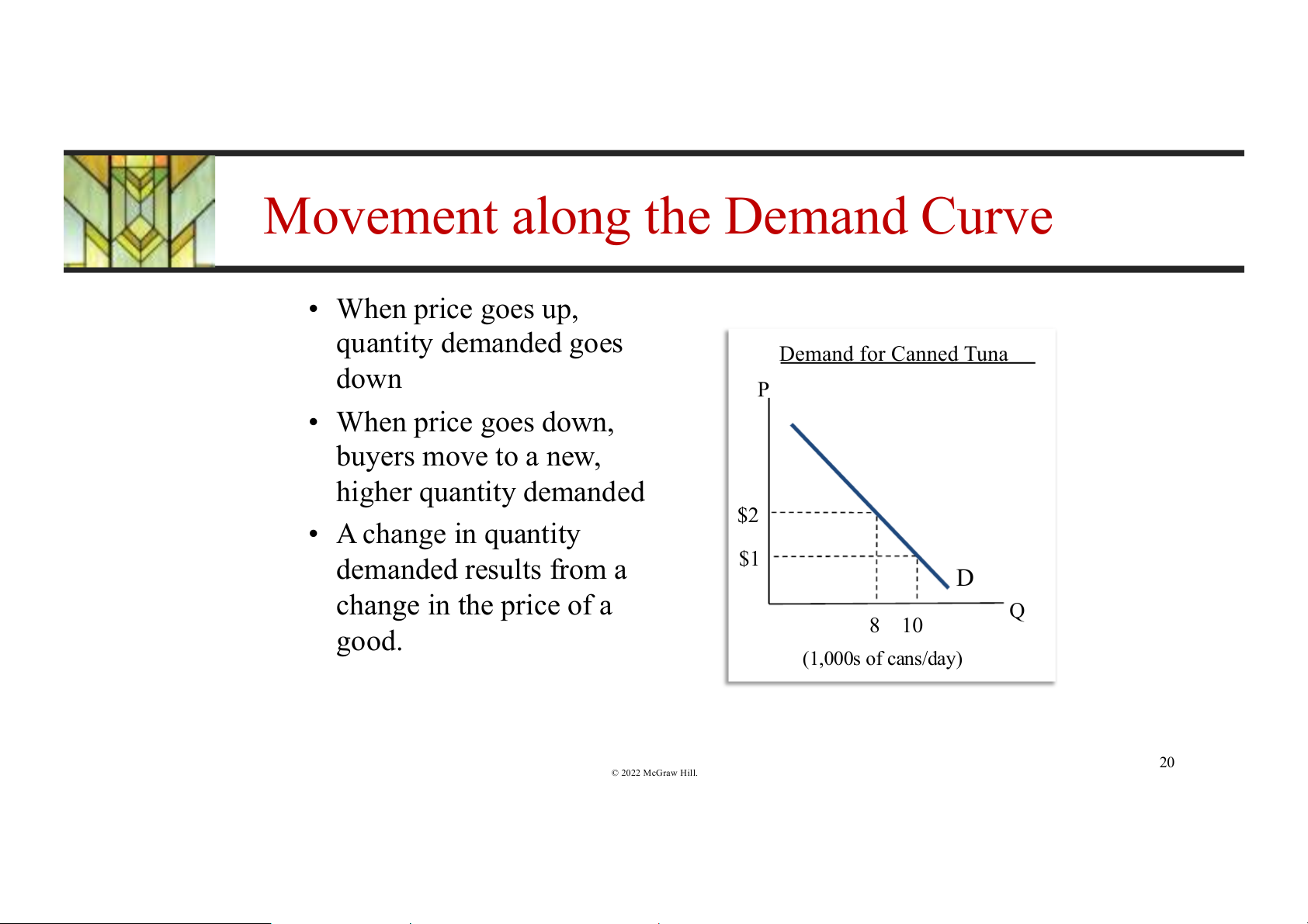
Movement along the Demand Curve • When price goes up, quantity demanded goes Demand for Canned Tuna down P • When price goes down, buyers move to a new, higher quantity demanded $2 • A change in quantity demanded results from a $1 D change in the price of a Q good. 8 10 (1,000s of cans/day) 20 © 2022 McGraw Hill.
Tài liệu liên quan:
-

Chương 3: độ co giãn và các nhân tố ảnh hưởng | Microeconomics | Trường Đại học Quốc tế, Đại học Quốc gia Thành phố Hồ Chí Minh
3 2 -
Microeconomics Syllabus | Microeconomics | Trường Đại học Quốc tế, Đại học Quốc gia Thành phố Hồ Chí Minh
3 2 -
Microeconomics Course Syllabus & Assessment Details | Microeconomics | Trường Đại học Quốc tế, Đại học Quốc gia Thành phố Hồ Chí Minh
3 2 -
Assignment 3 - Elasticity MCQs and Key Concepts | Microeconomics | Trường Đại học Quốc tế, Đại học Quốc gia Thành phố Hồ Chí Minh
3 2 -
Assignment 2 - Economic Equilibrium Analysis of Fridges and Motorcycles | Microeconomics | Trường Đại học Quốc tế, Đại học Quốc gia Thành phố Hồ Chí Minh
3 2