Bài giảng chương 10 : Integration | Môn toán cao cấp

Definition:Given a function f(x). If there  exists a function F(x) so that  F’(x) = f(x)  then F(x) is said to be the integral (also called anti-derivative or primitive) of f(x) and is written. Revising indefinite integration &  integrals of some simple functions. Tài liệu giúp bạn tham khảo, ôn tập và đạt kết quả cao. Mời bạn đọc đón xem !

lOMoARcPSD| 47207194 7/30/2020
1
Jacques,
Mathematics for Economics and Business
, 7
th
edition ' Pearson Education Limited 2012
Slide 6.1
Lecture 10
(28/4/2020)
Chapter 6
Integration
• Section 6.1. Indefinite integration & its applications in
economics and finance • Section 6.2. Definite
integration & its applications in economics and
finance
Jacques, Mathematics for Economics and Business, 7
th
edition ' Pearson Education Limited 2012
Slide 6.2
Section 6.1. Indefinite integration
Revising indefinite integration & integrals of some
simple functions
Finding the total (cost / revenue) function
given a marginal (cost / revenue) function
lOMoARcPSD| 47207194 7/30/2020
2
Jacques,
Mathematics for Economics and Business
, 7
th
edition ' Pearson Education Limited 2012
Finding consumption and savings functions
given MPC or MPS
Slide 6.3
Notation of indefinite integration
Definition: Given a function f(x). If there exists a function
F(x) so that
F’(x) = f(x)
then F(x) is said to be the integral (also called anti-derivative
or primitive) of f(x) and is written
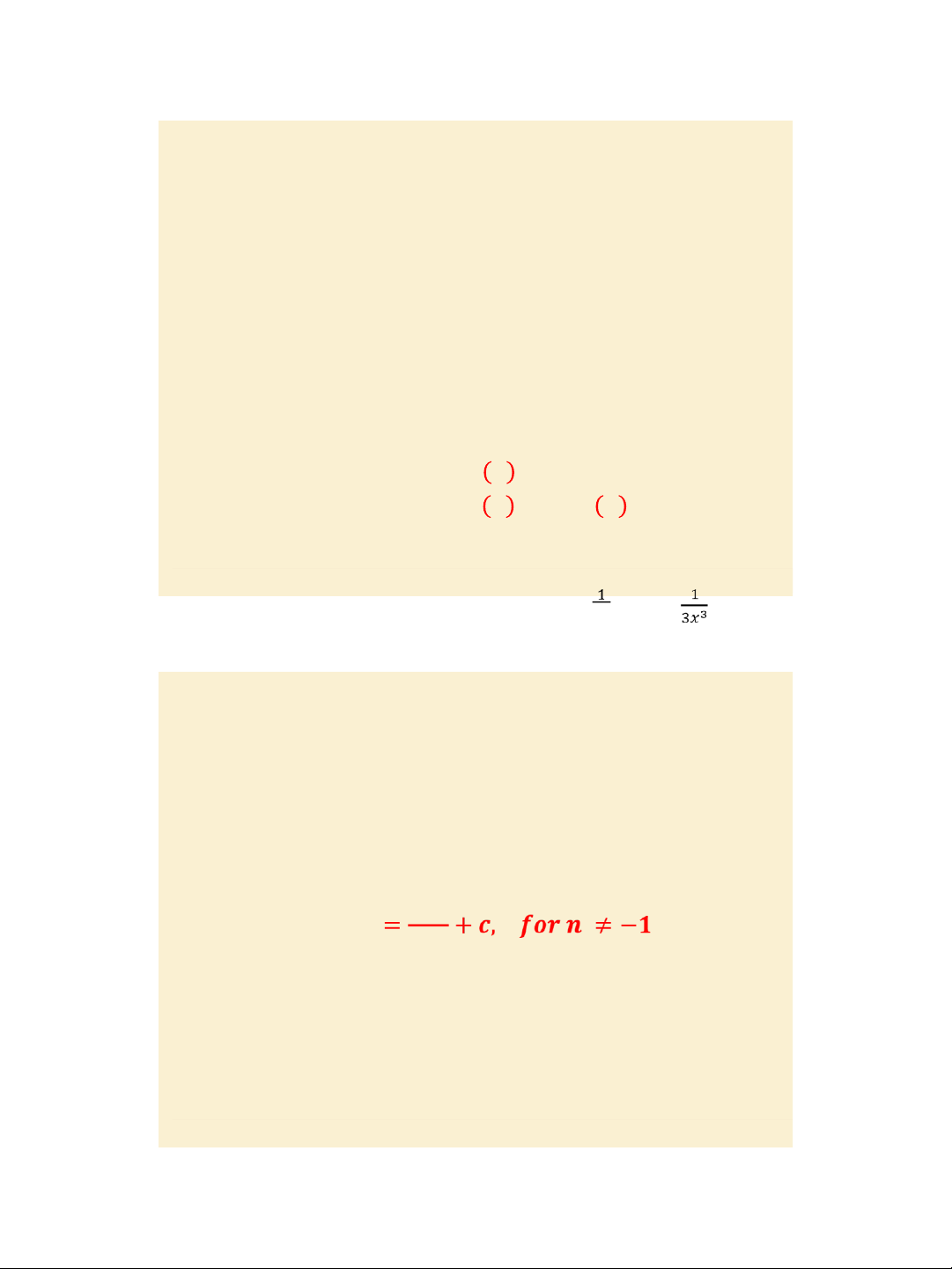
𝒇 𝒙 𝒅𝒙=𝑭(𝒙) We
then also have: 𝒇 𝒙 𝒅𝒙=𝑭 𝒙 +𝒄
since for any constant c, [F(x) + c]’ = f(x)
𝑑𝑥=− + c Example page 485: 3𝑥
2
𝑑𝑥= 𝑥
3
+ c,
𝑥
Jacques, Mathematics for Economics and Business, 7
th
edition ' Pearson Education Limited 2012
Slide 6.4
Indefinite integration of power and exponential functions,
and of a sum or difference of two functions
𝒏𝒅𝒙 𝒙𝒏+𝟏
𝒙 𝒏:𝟏
4
lOMoARcPSD| 47207194 7/30/2020
3
Jacques,
Mathematics for Economics and Business
, 7
th
edition ' Pearson Education Limited 2012
1
𝟏
𝒙
𝒅𝒙=𝒍𝒏𝒙+𝒄
𝒆𝒎𝒙𝒅𝒙 𝒎𝟏𝒆𝒎𝒙+𝒄
𝒂𝒇(𝒙𝒃𝒈(𝒙) 𝒅𝒙=𝒂 𝒇 𝒙𝒅𝒙 ±𝒃 𝒈 𝒙 𝒅𝒙
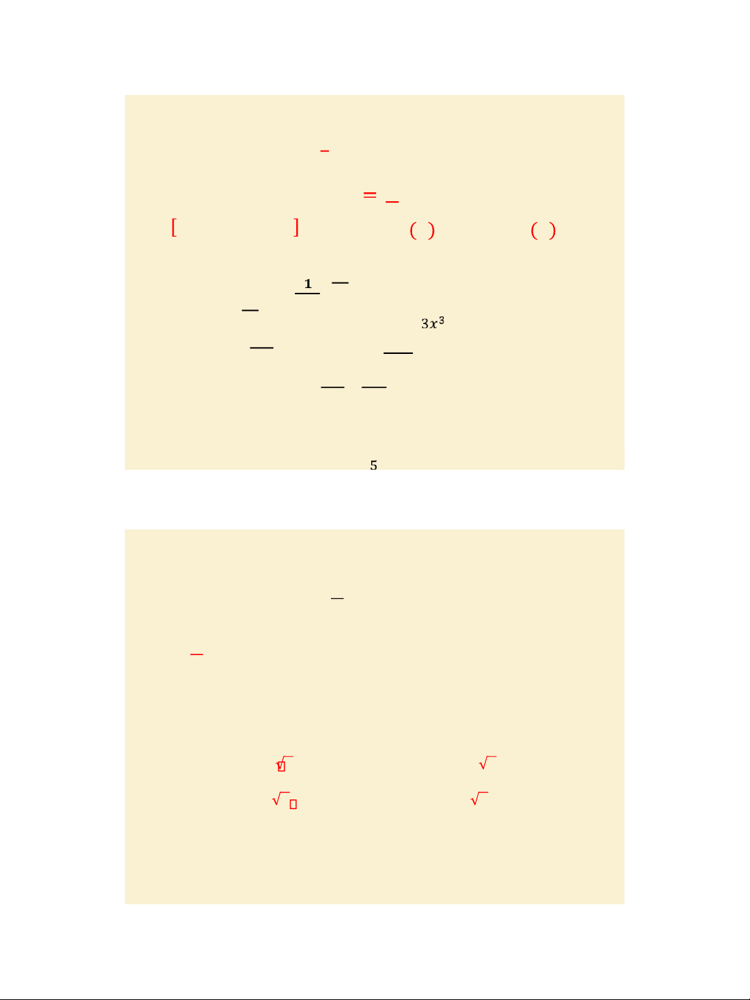
Example and practice problem, pages 487-490: 𝑥
4
𝑑𝑥=
𝑥
5
5
+ c,
𝑥
𝑑𝑥=− + c,
𝑒2𝑥𝑑𝑥= 𝑒22𝑥 + c, 𝑥1/3𝑑𝑥= 𝑥44//33 + c,
[2𝑒
4𝑥
−3𝑥
4
]𝑑𝑥=
𝑒
2
4𝑥
-
3𝑥
5
+ c.
Slide 6.5
Applications of indefinite integration in economics
Example, pages 491-493:
a/ Given a firm’s marginal cost function MC = Q
2
+ 2Q + 4, and the fixed
cost FC = 100. Find the total cost function TC.
MC = TC’ so TC = 𝑀𝐶 𝑑𝑄=
𝑄
3
3
+𝑄
2
+4𝑄+𝑐.
Since FC = 100 is TC at level Q = 0, we have c = 100, so:
TC =
𝑸𝟑
+𝑸
𝟐
+𝟒𝑸+𝟏𝟎𝟎.
𝟑
b/ MR function of a monopolist producer is MR = 10 – 4Q . MR = TR’ so
TR = 𝑀𝑅 𝑑𝑄= 10𝑄−2𝑄
2
+𝑐.
Since TR = 0 at level Q = 0, we have c = 0, so TR = 10Q – 2Q
2
.
Moreover, P = TR/Q implies P = 10 - 2Q. c/
MPC = 0.5 + 0.1/ 𝒀 C = 𝑴𝑷𝑪dY = 0.5Y + 0.2 𝒀 + c. If C =
85 when Y = 100 then c = 33.
d/ MPS = 0.4 - 0.1/ 𝒀 S = 𝑴𝑷𝑺dY = 0.4Y - 0.2 𝒀 + c. If S
= 0 when Y = 100 then c = - 38.
lOMoARcPSD| 47207194 7/30/2020
4
Jacques,
Mathematics for Economics and Business
, 7
th
edition ' Pearson Education Limited 2012
Key terms: page 495, Exercise 6.1*: problems 2, 4, 6, 7,12
pages 497 – 498.
Jacques, Mathematics for Economics and Business, 7
th
edition ' Pearson Education Limited 2012
Slide 6.6
Section 6.2. Definite integration
Revising definite integration & definite integrals of
some simple functions
Calculating the consumers surplus and
the producers surplus
Calculating the capital stock formation and present
value of a continuous revenue stream
Slide 6.7
lOMoARcPSD| 47207194 7/30/2020
5
Jacques,
Mathematics for Economics and Business
, 7
th
edition ' Pearson Education Limited 2012
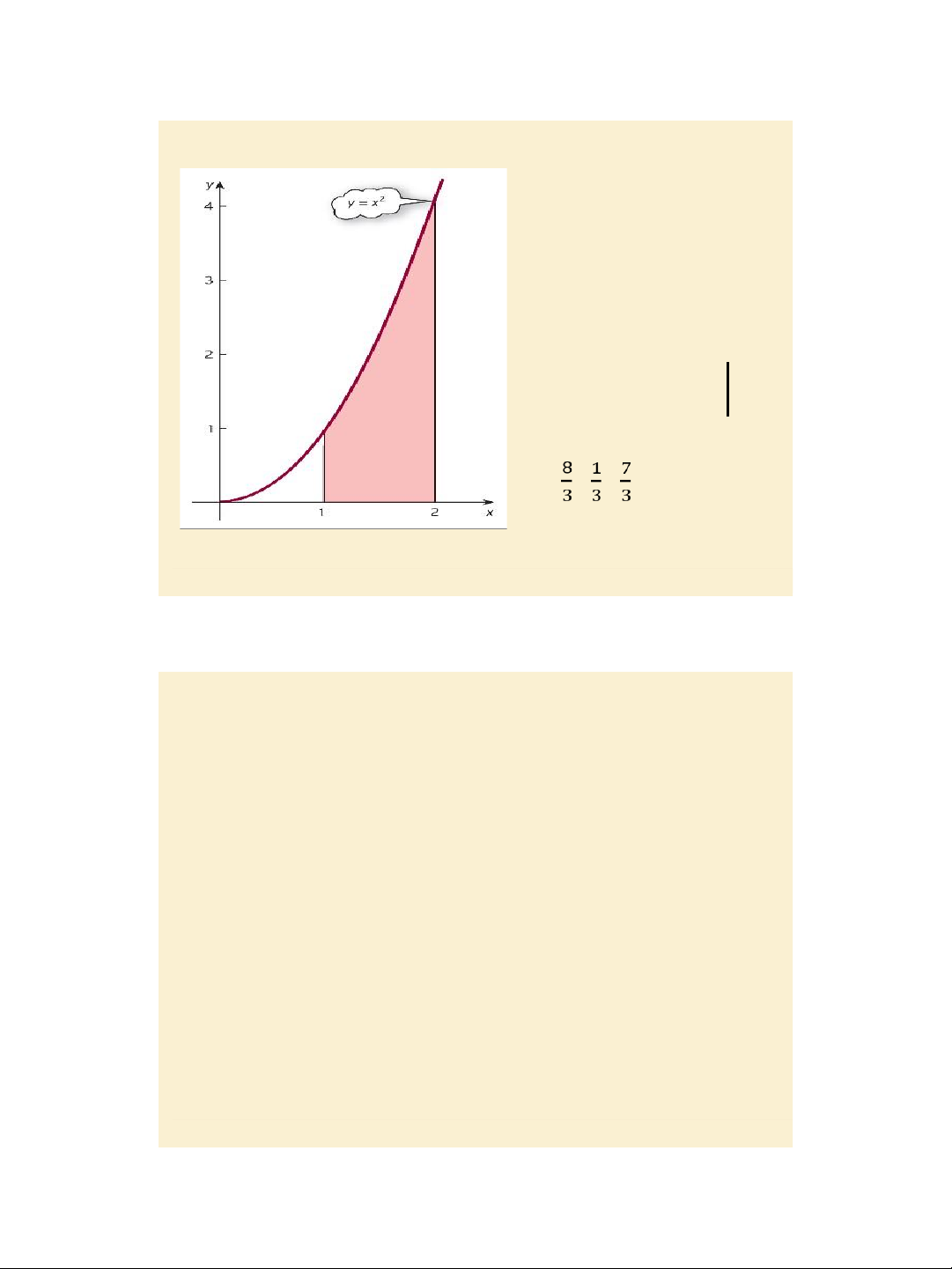
Finding the area of the
region bounded by the
curve y = x
2
, and
the lines x = 1
and x = 2.
2
S = 2𝑥2dx = 𝑥3
1 3
1
S = = .
Figure 6.1
Jacques, Mathematics for Economics and Business, 7
th
edition ' Pearson Education Limited 2012
Slide 6.8
lOMoARcPSD| 47207194 7/30/2020
6
Jacques,
Mathematics for Economics and Business
, 7
th
edition ' Pearson Education Limited 2012
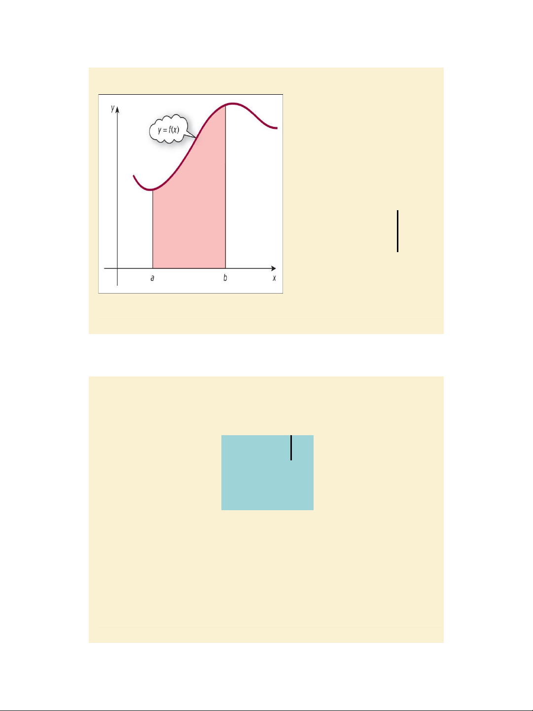
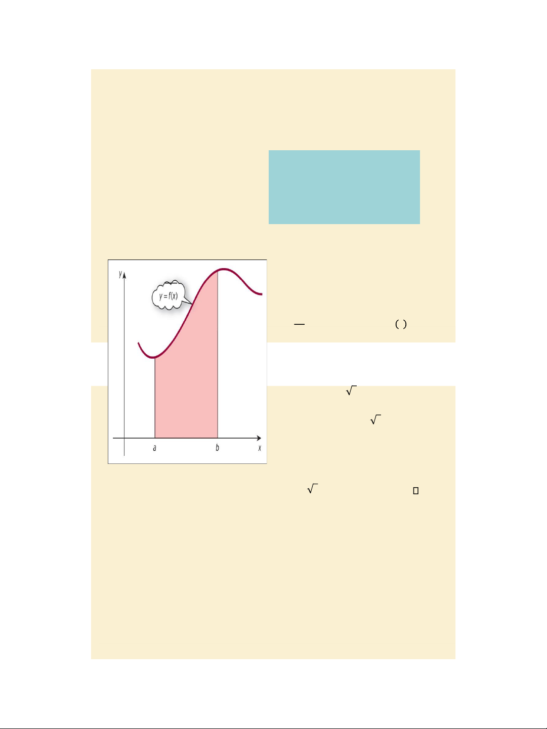
Concept of the definite
integral:
Finding the area under the
graph y = f(x) between x =
a and x = b.
(assuming f(x) ≥ 0 for all x
between a and b)
𝑏
𝑏
𝑎
𝑓(𝑥)dx = F(x)
𝑎
= F(b) – F(a), Where
a, b are the limits of
integration.
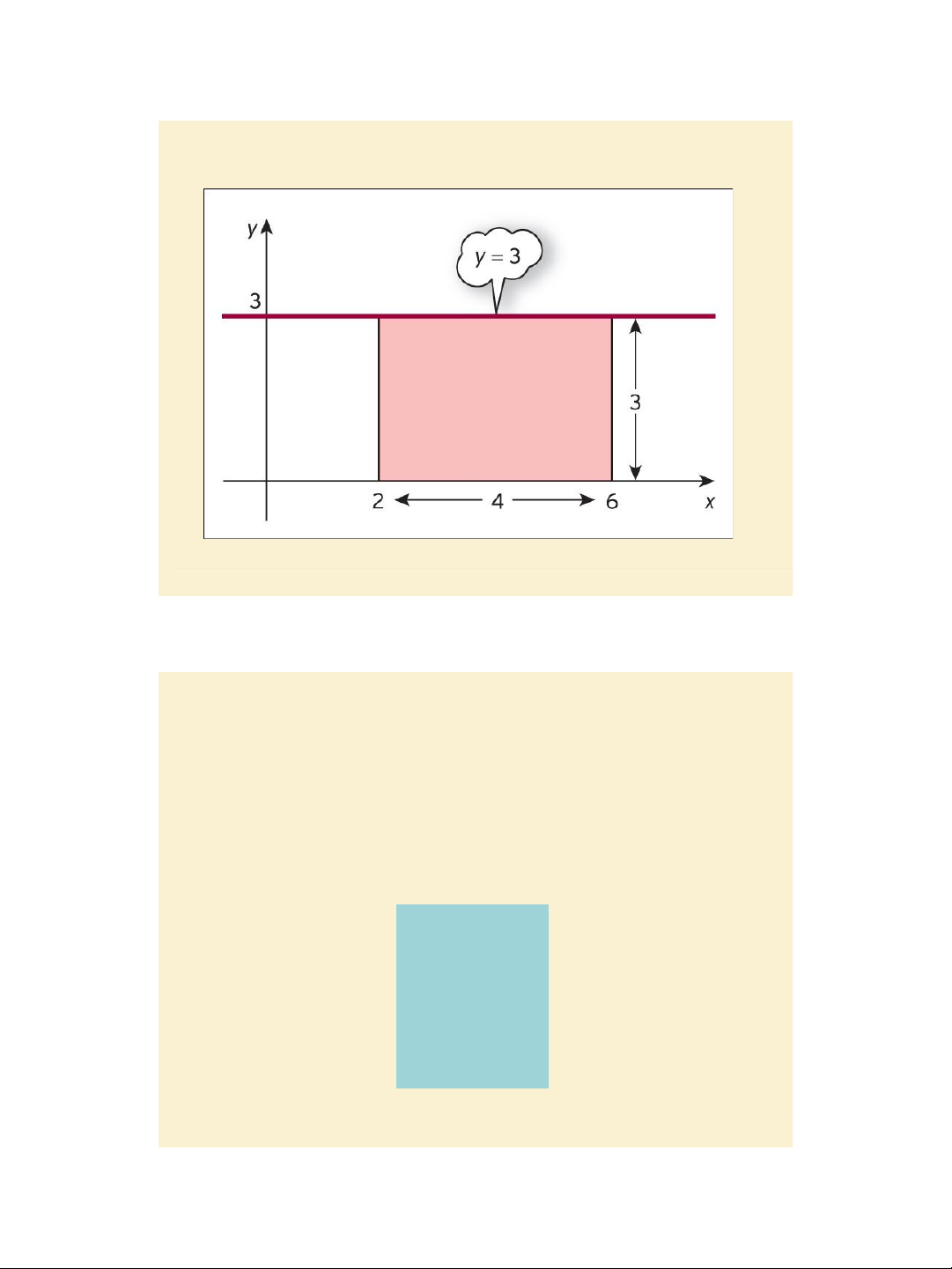
Figure 6.2
𝟐
𝟔
𝟑dx =
3x
𝟔
𝟐
= 18 – 6 = 12
lOMoARcPSD| 47207194 7/30/2020
7
Jacques,
Mathematics for Economics and Business
, 7
th
edition ' Pearson Education Limited 2012
Slide 6.9
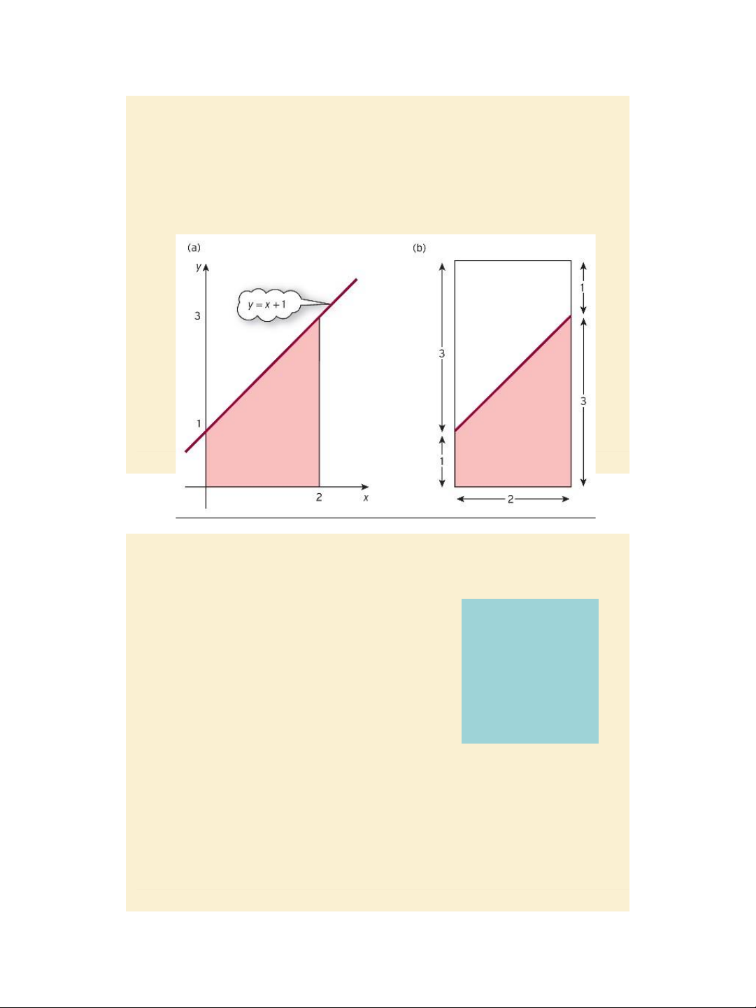
Figure 6.3
𝟎
𝟐
(𝒙+𝟏)dx =
𝟐
𝒙𝟐
+ 𝒙 =
𝟐
𝟎
= 4 – 0 = 4
lOMoARcPSD| 47207194 7/30/2020
8
Jacques,
Mathematics for Economics and Business
, 7
th
edition ' Pearson Education Limited 2012
Jacques, Mathematics for Economics and Business, 7
th
edition ' Pearson Education Limited 2012
Slide 6.10
Figure 6.4
Slide 6.11
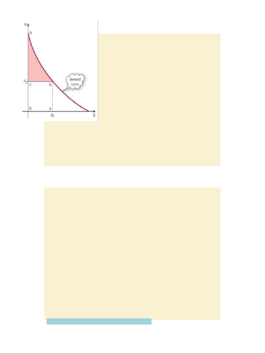
Calculating the consumer’s
surplus
Given the demand function /
demand curve P = f(Q).
The total amount of money spent on
Q
0
is Q
0
P
0
, where P
0
is the price that
consumers pay for the last unit i.e.
(id est: that is) Q
0
th
good.
For quantities up to Q
0
, consumers
would be willing to pay the higher
price given by the demand curve.
The shaded area BCD represents
the benefit to the consumer of
paying the fixed price P
0
and is
called the consumer’s surplus:
CS =
𝟎
𝑸
𝟎
𝒇(𝑸)dQ
– Q
0
P
0
Figure 6.5
Example, page 503:
Find the consumer’s
surplus at Q
0
= 5 for
demand function P =
30 – 4Q.
P
0
= 30 - 4ₓ5 = 10
CS =
𝟎
𝟓
(𝟑𝟎𝟒𝑸)dQ
lOMoARcPSD| 47207194 7/30/2020
9
Jacques,
Mathematics for Economics and Business
, 7
th
edition ' Pearson Education Limited 2012
Jacques, Mathematics for Economics and Business, 7
th
edition ' Pearson Education Limited 2012
Slide 6.12
Calculating the producer’s
surplus
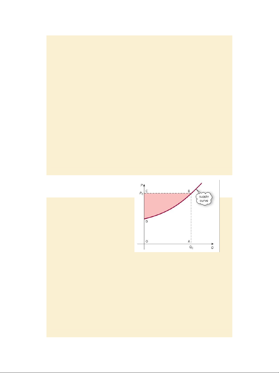
Given the supply function / supply
curve P = g(Q). At Q = Q
0
, P = P
0
.
If all quantity Q
0
is sold, the total
amount of money received is
Q
0
P
0
. Note that P
0
is the price that
the producers supply for the last
unit i.e. Q
0
th
good.
For quantities up to Q
0
, producers
would be willing to supply the lower price
given by the supply curve. Figure 6.6
lOMoARcPSD| 47207194 7/30/2020
10
Jacques,
Mathematics for Economics and Business
, 7
th
edition ' Pearson Education Limited 2012
– 5ₓ10 = 50
lOMoARcPSD| 47207194 7/30/2020
11
Jacques,
Mathematics for Economics and Business
, 7
th
edition ' Pearson Education Limited 2012
formation:
I(t) =
𝑑𝐾
𝑑𝑡
I (t) =
𝒅𝑲
𝒅𝒕
I
t
2
t
t
1
The shaded area BCD
represents the benefit to the
producer of selling goods of the
fixed price P
0
and is called the
producer’s surplus:
PS = Q
0
P
0
-
𝟎
𝑸
𝟎
𝒈(𝑸)dQ
Example, page 505: Find the
producer’s surplus at Q
0
= 4 for
supply function P = 3 + Q
2
. P
0
=
3 + 4ₓ4 = 19
PS = 4ₓ19
𝟎
𝟒
(𝟑+𝑸
𝟐
)dQ = 42
𝟐
𝟑
Slide 6.13
Calculating the capital stock
The rate of net investment flow I(t) is
the rate of change of capital stock K
per time period:
= K’(t). So K(t) = 𝐼 𝑡 𝑑𝑡 & the
capital stock formation between t
1
and
t
2
is:
𝑡
𝑡
1
2
𝐼(𝑡)dt = K(t
2
) – K(t
1
).
Example, page 507:
Given I(t) = 9000 𝑡.
a/ The capital formation between year
1 and year 4 is:
1
4
9000 𝑡dt = $42000.
b/ The number of years required before
the capital stock first exceeds 100000:
0
𝑇
9000𝑡dt = 6000T
3/2
= 100000 T =
6.5.
Jacques, Mathematics for Economics and Business, 7
th
edition ' Pearson Education Limited 2012
Slide 6.14
lOMoARcPSD| 47207194 7/30/2020
12
Jacques,
Mathematics for Economics and Business
, 7
th
edition ' Pearson Education Limited 2012
The present value of a continuous revenue stream
In chapter 3, section 3.4, we learned that to discount a future value S to
present value S
0
, the following formula can be used:
𝑺
𝟎
=𝑺𝒆
;𝒓𝒏/𝟏𝟎𝟎
for continuous compounding, where r (%) is the nominal rate of
interest, n is number years the interest is compounded.
Consider a fund formed by an annuity / a continuous revenue stream with
an annual rate S dollars per year. Using the above discounting formula,
the present value of fund is:
𝑷= 𝑺𝒆;𝒓𝒕
𝟏
/𝟏𝟎𝟎 ×𝜟𝒕
𝟏
+𝑺𝒆;𝒓𝒕
𝟐
/𝟏𝟎𝟎 ×𝜟𝒕
𝟐
; 𝒓𝒕𝒒/𝟏𝟎𝟎𝜟𝒕
𝒒
For the sake of simple interpretation, the continuous revenue stream is
considered like a discrete revenue stream, with rate S/52 dollars per
week. Then, in the above formula:
Δt
i
= 1/52 for i = 1, ..., q, with q = 52n and t
1
= 1/52, t
i+1
= t
i
+ 1/52 for
According to the definition of the definite integral: 𝑷=
𝟎
𝒏 𝑺𝒆; 𝟏𝟎𝟎𝒓𝒕 𝒅𝒕 .
Example, page 508: Calculate the present value of a continuous revenue
stream for 5 years at a constant rate $1000 per year if the discount rate is
9%.
Slide 6.15
The present value of a continuous revenue stream
𝒏
;
𝟏𝟎𝟎𝒓𝒕 𝒅𝒕
𝑷 = 𝑺 𝒆
𝟎
Example, page 508: Calculate the present value of a
continuous revenue stream for 5 years at a constant rate
$1000 per year if the discount rate is 9%.
Using the above formula: 𝑃=
0
5
1000𝑒
;0.09𝑡
𝑑𝑡 = $ 4026.35.
Practice problem: page 508.
lOMoARcPSD| 47207194 7/30/2020
13
Jacques,
Mathematics for Economics and Business
, 7
th
edition ' Pearson Education Limited 2012
Key terms: page 509,
Exercise 6.2*: problems 2, 3, 4, 6, 7, 9 pages 510 - 511
Jacques, Mathematics for Economics and Business, 7
th
edition ' Pearson Education Limited 2012
Slide 6.16
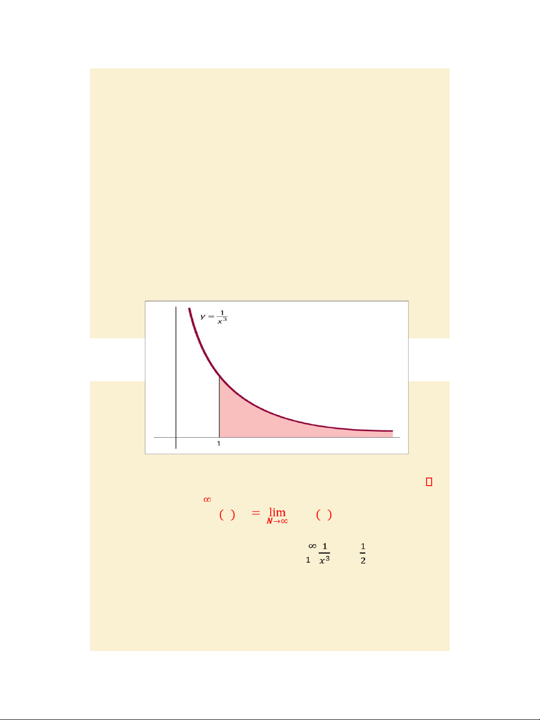
Figure 6.7
Formal Maths: The definite integral with the upper limit +
𝑵
𝒇 𝒙 𝒅𝒙 𝒇 𝒙 𝒅𝒙
𝒂𝒂
Example, pages 513 – 514: Evaluate 𝑑𝑥 =
| 1/13

Preview text:

7/30/2020 lOMoAR cPSD| 47207194 Slide 6.1 Lecture 10 (28/4/2020) Chapter 6 Integration
• Section 6.1. Indefinite integration & its applications in
economics and finance • Section 6.2. Definite
integration & its applications in economics and finance
Jacques, Mathematics for Economics and Business, 7th edition ' Pearson Education Limited 2012 Slide 6.2
Section 6.1. Indefinite integration
Revising indefinite integration & integrals of some simple functions
Finding the total (cost / revenue) function
given a marginal (cost / revenue) function
Jacques, Mathematics for Economics and Business , 7 th edition ' Pearson Education Limited 2012 1 7/30/2020 lOMoAR cPSD| 47207194
Finding consumption and savings functions given MPC or MPS Slide 6.3
Notation of indefinite integration
Definition: Given a function f(x). If there exists a function F(x) so that
F’(x) = f(x)
then F(x) is said to be the integral (also called anti-derivative
or primitive) of f(x) and is written
𝒇 𝒙 𝒅𝒙=𝑭(𝒙) We
then also have: 𝒇 𝒙 𝒅𝒙=𝑭 𝒙 +𝒄
since for any constant c, [F(x) + c]’ = f(x)
Example page 485: 3𝑥2𝑑𝑥= 𝑥3 + c, 4 𝑥 𝑑𝑥=− + c
Jacques, Mathematics for Economics and Business, 7th edition ' Pearson Education Limited 2012 Slide 6.4
Indefinite integration of power and exponential functions,
and of a sum or difference of two functions 𝒏𝒅𝒙 𝒙𝒏+𝟏 𝒙 𝒏:𝟏
Jacques, Mathematics for Economics and Business , 7 th edition ' Pearson Education Limited 2012 2 7/30/2020 lOMoAR cPSD| 47207194
𝟏𝒙𝒅𝒙=𝒍𝒏𝒙+𝒄
𝒆𝒎𝒙𝒅𝒙 𝒎𝟏𝒆𝒎𝒙+𝒄
𝒂𝒇(𝒙)±𝒃𝒈(𝒙) 𝒅𝒙=𝒂 𝒇 𝒙𝒅𝒙 ±𝒃 𝒈 𝒙 𝒅𝒙
Example and practice problem, pages 487-490: 𝑥4𝑑𝑥= 1 𝑥55 + c, 𝑥 𝑑𝑥=− 4 + c,
𝑒2𝑥𝑑𝑥= 𝑒22𝑥 + c, 𝑥1/3𝑑𝑥= 𝑥44//33 + c,
[2𝑒4𝑥 −3𝑥4]𝑑𝑥= 𝑒24𝑥 - 3𝑥5 + c. Slide 6.5
Applications of indefinite integration in economics Example, pages 491-493:
a/ Given a firm’s marginal cost function MC = Q2 + 2Q + 4, and the fixed
cost FC = 100. Find the total cost function TC.
MC = TC’ so TC = 𝑀𝐶 𝑑𝑄= 𝑄33+𝑄2 +4𝑄+𝑐.
Since FC = 100 is TC at level Q = 0, we have c = 100, so:
TC = 𝑸𝟑 +𝑸𝟐 +𝟒𝑸+𝟏𝟎𝟎. 𝟑
b/ MR function of a monopolist producer is MR = 10 – 4Q . MR = TR’ so
TR = 𝑀𝑅 𝑑𝑄= 10𝑄−2𝑄2 +𝑐.
Since TR = 0 at level Q = 0, we have c = 0, so TR = 10Q – 2Q2.
Moreover, P = TR/Q implies P = 10 - 2Q. c/
MPC = 0.5 + 0.1/ 𝒀 C = 𝑴𝑷𝑪dY = 0.5Y + 0.2 𝒀 + c. If C = 85 when Y = 100 then c = 33.
d/ MPS = 0.4 - 0.1/ 𝒀 S = 𝑴𝑷𝑺dY = 0.4Y - 0.2 𝒀 + c. If S
= 0 when Y = 100 then c = - 38.
Jacques, Mathematics for Economics and Business , 7 th edition ' Pearson Education Limited 2012 3 7/30/2020 lOMoAR cPSD| 47207194
Key terms: page 495, Exercise 6.1*: problems 2, 4, 6, 7,12 pages 497 – 498.
Jacques, Mathematics for Economics and Business, 7th edition ' Pearson Education Limited 2012 Slide 6.6
Section 6.2. Definite integration
Revising definite integration & definite integrals of some simple functions
Calculating the consumer’s surplus and
the producer’s surplus
Calculating the capital stock formation and present
value of a continuous revenue stream Slide 6.7
Jacques, Mathematics for Economics and Business , 7 th edition ' Pearson Education Limited 2012 4 7/30/2020 lOMoAR cPSD| 47207194 Finding the area of the region bounded by the curve y = x2, and the lines x = 1 and x = 2. 2 S = 2𝑥2dx = 𝑥3 1 3 1 S = − = . Figure 6.1
Jacques, Mathematics for Economics and Business, 7th edition ' Pearson Education Limited 2012 Slide 6.8
Jacques, Mathematics for Economics and Business , 7 th edition ' Pearson Education Limited 2012 5 7/30/2020 lOMoAR cPSD| 47207194 Concept of the definite integral: Finding the area under the graph y = f(x) between x = a and x = b.
(assuming f(x) ≥ 0 for all x between a and b) 𝑏 𝑏 𝑎 𝑓(𝑥)dx = F(x) 𝑎 = F(b) – F(a), Where a, b are the limits of integration. Figure 6.2 𝟐𝟔𝟑dx = 3x 𝟔 𝟐 = 18 – 6 = 12
Jacques, Mathematics for Economics and Business , 7 th edition ' Pearson Education Limited 2012 6 7/30/2020 lOMoAR cPSD| 47207194 Slide 6.9 Figure 6.3
𝟎𝟐(𝒙+𝟏)dx = 𝟐 𝒙𝟐 + 𝒙 = 𝟐 𝟎 = 4 – 0 = 4
Jacques, Mathematics for Economics and Business , 7 th edition ' Pearson Education Limited 2012 7 7/30/2020 lOMoAR cPSD| 47207194
Jacques, Mathematics for Economics and Business, 7th edition ' Pearson Education Limited 2012 Slide 6.10 Figure 6.4 Slide 6.11
CS = 𝟎𝑸𝟎𝒇(𝑸)dQ
Calculating the consumer’s – Q0P0 surplus Figure 6.5 Example, page 503: Given the demand function / Find the consumer’s demand curve P = f(Q). surplus at Q0 = 5 for
The total amount of money spent on demand function P =
Q0 is Q0P0, where P0 is the price that 30 – 4Q.
consumers pay for the last unit i.e. (id est: that is) Q P0 = 30 - 4ₓ5 = 10 0th good.
For quantities up to Q0, consumers
CS = 𝟎𝟓(𝟑𝟎−𝟒𝑸)dQ
would be wil ing to pay the higher
price given by the demand curve.
The shaded area BCD represents
the benefit to the consumer of
paying the fixed price P0 and is
called the consumer’s surplus:
Jacques, Mathematics for Economics and Business , 7 th edition ' Pearson Education Limited 2012 8 7/30/2020 lOMoAR cPSD| 47207194
Jacques, Mathematics for Economics and Business, 7th edition ' Pearson Education Limited 2012 Slide 6.12
Calculating the producer’s surplus
Given the supply function / supply
curve P = g(Q). At Q = Q0, P = P0.
If all quantity Q0 is sold, the total amount of money received is
Q0P0. Note that P0 is the price that
the producers supply for the last unit i.e. Q0th good.
For quantities up to Q0, producers
would be wil ing to supply the lower price given by the supply curve. Figure 6.6
Jacques, Mathematics for Economics and Business , 7 th edition ' Pearson Education Limited 2012 9 7/30/2020 lOMoAR cPSD| 47207194
Jacques, Mathematics for Economics and Business , 7 th edition ' Pearson Education Limited 2012
– 5ₓ10 = 50 10 7/30/2020 lOMoAR cPSD| 47207194 The shaded area BCD
PS = Q0P0 - 𝟎𝑸𝟎𝒈(𝑸)dQ represents the benefit to the
Example, page 505: Find the
producer of selling goods of the
producer’s surplus at Q0 = 4 for
fixed price P0 and is called the
supply function P = 3 + Q2. P0 = producer’s surplus: 3 + 4ₓ4 = 19
PS = 4ₓ19 − 𝟎𝟒(𝟑+𝑸𝟐)dQ = 42𝟐𝟑 Slide 6.13
Calculating the capital stock formation:
I I (t) = 𝒅𝑲
The rate of net investment flow I(t) is 𝒅𝒕
the rate of change of capital stock K per time period:
I(t) = 𝑑𝐾 = K’(t). So K(t) = 𝐼 𝑡 𝑑𝑡 & the 𝑑𝑡
capital stock formation between t1 and
t2 is: 𝑡𝑡12𝐼(𝑡)dt = K(t2) – K(t1). Example, page 507: Given I(t) = 9000 𝑡.
a/ The capital formation between year
1 and year 4 is: 149000 𝑡dt = $42000. t t 1 2 t
b/ The number of years required before
the capital stock first exceeds 100000:
0𝑇9000𝑡dt = 6000T3/2 = 100000 T = 6.5.
Jacques, Mathematics for Economics and Business, 7th edition ' Pearson Education Limited 2012 Slide 6.14
Jacques, Mathematics for Economics and Business , 7 th edition ' Pearson Education Limited 2012 11 7/30/2020 lOMoAR cPSD| 47207194
The present value of a continuous revenue stream
In chapter 3, section 3.4, we learned that to discount a future value S to
present value S0, the fol owing formula can be used:
𝑺𝟎 =𝑺𝒆;𝒓𝒏/𝟏𝟎𝟎 for continuous compounding, where r (%) is the nominal rate of
interest, n is number years the interest is compounded.
Consider a fund formed by an annuity / a continuous revenue stream with
an annual rate S dollars per year. Using the above discounting formula, the present value of fund is:
𝑷= 𝑺𝒆;𝒓𝒕𝟏/𝟏𝟎𝟎 ×𝜟𝒕𝟏+𝑺𝒆;𝒓𝒕𝟐/𝟏𝟎𝟎 ×𝜟𝒕𝟐
; 𝒓𝒕𝒒/𝟏𝟎𝟎𝜟𝒕𝒒
For the sake of simple interpretation, the continuous revenue stream is
considered like a discrete revenue stream, with rate S/52 dollars per
week. Then, in the above formula:
Δti = 1/52 for i = 1, ..., q, with q = 52n and t1 = 1/52, ti+1 = ti + 1/52 for
According to the definition of the definite integral: 𝑷= 𝟎𝒏 𝑺𝒆; 𝟏𝟎𝟎𝒓𝒕 𝒅𝒕 .
Example, page 508: Calculate the present value of a continuous revenue
stream for 5 years at a constant rate $1000 per year if the discount rate is 9%. Slide 6.15
The present value of a continuous revenue stream 𝒏
; 𝟏𝟎𝟎𝒓𝒕 𝒅𝒕 𝑷 = 𝑺 𝒆 𝟎
Example, page 508: Calculate the present value of a
continuous revenue stream for 5 years at a constant rate
$1000 per year if the discount rate is 9%.
Using the above formula: 𝑃= 05 1000𝑒;0.09𝑡 𝑑𝑡 = $ 4026.35. Practice problem: page 508.
Jacques, Mathematics for Economics and Business , 7 th edition ' Pearson Education Limited 2012 12 7/30/2020 lOMoAR cPSD| 47207194 Key terms: page 509,
Exercise 6.2*: problems 2, 3, 4, 6, 7, 9 pages 510 - 511
Jacques, Mathematics for Economics and Business, 7th edition ' Pearson Education Limited 2012 Slide 6.16 Figure 6.7
Formal Maths: The definite integral with the upper limit + 𝑵 𝒇 𝒙 𝒅𝒙 𝒇 𝒙 𝒅𝒙 𝒂𝒂
Example, pages 513 – 514: Evaluate 𝑑𝑥 =
Jacques, Mathematics for Economics and Business , 7 th edition ' Pearson Education Limited 2012 13