Bài giảng chương 14: Dynamics | Môn toán cao cấp

7/31/2020 lOMoAR cPSD| 47207194 Slide 9.1 Lecture 14 (26/5/2020) Chapter 9 Dynamics Slide 9.2 Section 9.1. Difference equations
Find the complementary function and the
particular solution of a difference equation
Analyze the stability of economic systems
Solve lagged national income determination models and
single-commodity-market models with lagged supply
Jacques, Mathematics for Economics and Business , 7 th edition ' Pearson Education Limited 2012 1 7/31/2020 lOMoAR cPSD| 47207194
• Section 9.1. Difference equations
Jacques, Mathematics for Economics and Business, 7th edition ' Pearson Education Limited 2012
Jacques, Mathematics for Economics and Business , 7 th edition ' Pearson Education Limited 2012 2 7/31/2020 lOMoAR cPSD| 47207194 Slide 9.3
Concept of difference equations
Consider national income in year t, which is denoted by Yt and is an
economic variable depending on t. Suppose the growth rate of national
income is 7% per year, then Y1 = 1.07Y0, Y2 = 1.07Y1, Y3 = 1.07Y2, …, Yt
= 1.07 Yt-1, … As learned before, the sequence Y0, Y1, Y2, Y3, …., Yt, …
is a geometric progression with the geometric ratio 1.07. The equation Yt = 1.07Yt-1 relates Yt to Yt-1.
Definition: A difference equation is an equation that relates
consecutive terms of sequence of numbers.
Example, page 628: Consider the difference equation Yt = 2Yt-1 . Let Y0 =
3, the first four terms of the sequence are Y0 = 3, Y1 = 2Y0 = 2 3 = 6, Y2 = 2Y1 = 22 3 =12, Y3 = 2Y2 = 23 3 = 24,
and the general term of sequence is: Yt = 2Yt-1= 2t 3. Slide 9.4
Solution of difference equation: Yt = bYt-1 + c with Y0 = y0 (*)
(the 1st order linear difference equation)
Step 1. Finding the solution of d.e. Yt = bYt-1. The solution is Yt = Abt
(for any value of constant A)
This solution is called the complementary function for d.e. (*) and denoted by CF.
Step 2. Finding a particular solution of difference equation Yt = bYt-1 + c.
A particular solution is denoted by PS and can be found by the formula Yt = c/(1-b) if b 1 or Yt = ct if b = 1.
Step 3. Solving difference equation Yt = bYt-1 + c. The general solution is Yt = CF + PS.
Case 1, b 1: Yt = Abt + c/(1-b) Case 2, b = 1: Yt = A + ct.
Step 4. Choose A to satisfy the initial condition Y0 = y0.
Case 1, b 1: A = y0 – c/(1-b) Case 2, b = 1: A = y0
Jacques, Mathematics for Economics and Business , 7 th edition ' Pearson Education Limited 2012 3 7/31/2020 lOMoAR cPSD| 47207194
It is said that Yt = 3 2t is the solution of the difference equation Yt =
2Yt-1 with initial condition Y0 = 3. In general, Yt = y0bt is the solution
of the difference equation Yt = bYt-1 with initial condition Y0 = y0.
Jacques, Mathematics for Economics and Business, 7th edition ' Pearson Education Limited 2012
Jacques, Mathematics for Economics and Business , 7 th edition ' Pearson Education Limited 2012 4 7/31/2020 lOMoAR cPSD| 47207194 Slide 9.5
Solution of difference equation:
Yt = bYt-1 + c with Y0 = y0 Example, pages 630 - 631:
Yt = 4Yt-1 + 21 with Y0 = 1 Step 1.
Finding the complementary function CF = A4t.
Step 2. Finding a particular solution PS = 21/(1 - 4) = - 7.
Step 3. Finding the general solution Yt = CF + PS = A4t - 7.
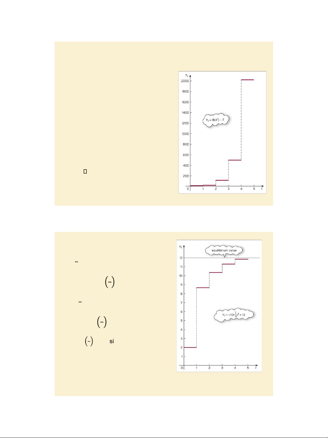
Step 4. The solution satisfying Y0 = 1 is
Yt = 8 4t - 7 (since A = 1 – (-7) = 8).
The graph of Yt is cal ed the time path
of economic variable Yt. In this case, it
is said that the time path diverges uniformly or explodes (since b = 4 > 1). Figure 9.1 Slide 9.6
Solution of difference equation: Example, pages 632 - 633: 1 Y = Y + 8 with Y = 2 t t-1 0 3
Step 1. Finding the complementary 1 function CF = A t . 3
Step 2. Finding a particular solution PS = 1 8 /(1 - ) = 12. 3
Step 3. Finding the general solution Y = t 1 CF + PS = A t + 12. 3
Step 4. The solution satisfying Y = 2 is 0
Y = - 10 1 t +12 (s ince A = 2 – 12 = -10). t 3
In this case, the time path of Y t
converges uniformly to the equilibrium
level 12 (since b = 1/3 < 1). Figure 9.2 Practice problem, page 633.
Jacques, Mathematics for Economics and Business , 7 th edition ' Pearson Education Limited 2012 5 7/31/2020 lOMoAR cPSD| 47207194
Jacques, Mathematics for Economics and Business, 7th edition ' Pearson Education Limited 2012
Jacques, Mathematics for Economics and Business , 7 th edition ' Pearson Education Limited 2012 6 7/31/2020 lOMoAR cPSD| 47207194 Slide 9.7
Classifying solutions of difference equations: Yt = bYt-1
+ c with Y0 = y0 and analyzing stability of the economic model
General solution Value of A to satisfy Y0 = y0 b 1 Yt = Abt + c/(1-b) A = y0 – c/(1-b) b = 1 Yt = A + ct. A = y0 Yt displays The model is b > 1 uniform divergence unstable 0 < b < 1 uniform convergence stable
-1 < b < 0 oscil atory convergence stable b < -1 oscil atory divergence unstable Slide 9.8
National income determination
Recall that in Chapter 1, section 1.7, we learned about the simple two-
sector macro-economic model with structural equations: Y = C + I C = aY + b I = I*.
In practice, there is a time lag between C and Y, that is consumption
in year t: Ct depends on national income in previous year t – 1: Yt-1 .
We can rewrite the above 03 equations as follows in the form of timedependent equations: Yt = Ct + It Ct = aYt-1 + b It = I*.
On substituting the expressions for Ct and It in the 1st equation, we
have the fol owing (1st order linear) difference equation:
Yt = aYt-1 + b + I* (**)
If Y0 is known then we can derive an expression for Yt explicitly by
solving d.e. (**) with the initial condition Y0 = y0.
Jacques, Mathematics for Economics and Business , 7 th edition ' Pearson Education Limited 2012 7 7/31/2020 lOMoAR cPSD| 47207194
Jacques, Mathematics for Economics and Business, 7th edition ' Pearson Education Limited 2012
Jacques, Mathematics for Economics and Business , 7 th edition ' Pearson Education Limited 2012 8 7/31/2020 lOMoAR cPSD| 47207194 Slide 9.9
National income determination Example, page 635: Consider a two-sector model Yt = Ct + It Ct = 0.8Yt-1 +100 It = 200.
Find an expression for Yt when Y0 = 1700.
On substituting the expressions for Ct and It in the 1st equation, we
have the following (1st order linear) difference equation: Yt = 0.8Yt-1 + 300
with the initial condition Y0 = 1700.
Applying the 4-step solution procedure we can derive the solution: Yt = 200 0.8t +1500.
As t (time) increases, 0.8t converges to 0, and hence Yt converges
to the equilibrium level 1500. The time path displays uniform Slide 9.10
Supply and demand analysis
Recall that in Chapter 1, section 1.5, we learned about the simple model
of supply and demand for a single good with structural equations: QS = aP - b QD = -cP + d QD = QS.
In practice, there is a time lag between QS and P, that is QS in period t:
QSt depends on P in previous period t – 1: Pt-1 . We can rewrite the
above 03 equations as fol ows in the form of time – dependent supply and demand equations:
QSt = aPt-1 - b QDt = -cPt + d QDt = QSt. 𝒂 It is easy to derive: aP +
t-1 – b = -cPt + d 𝑷𝒕 = −𝒄 𝑷𝒕−𝟏 𝒃+𝒅𝒄 (***).
If P0 is known then we can derive an expression for Pt explicitly by
solving d.e. (***) with the initial condition P0 = p0.
Moreover, we can also find an expression for Qt, since Qt = -cPt + d. If
c > a (> 0) then system is stable, else if a > c ( > 0) the system is unstable.
Jacques, Mathematics for Economics and Business , 7 th edition ' Pearson Education Limited 2012 9 7/31/2020 lOMoAR cPSD| 47207194
convergence. The given system / economic model is stable. Note
that MPC = 0.8 implies stability of the model.
Jacques, Mathematics for Economics and Business, 7th edition ' Pearson Education Limited 2012
Jacques, Mathematics for Economics and Business , 7 th edition ' Pearson Education Limited 2012 10 7/31/2020 lOMoAR cPSD| 47207194 Slide 9.11
Supply and demand analysis Example, page 637:
Consider the supply and demand equations QSt = 4Pt-1 - 10 QDt = -5Pt + 35.
Assuming that the market is in equilibrium, find expressions for Pt
and Qt when P0 = 6. Is the system stable?
It is easy to get the following (1st order linear) difference equation: Pt = -0.8Pt-1 + 9 with the initial condition P0 = 6.
Applying the 4-step solution procedure we can derive the solution:
Pt = (-0.8)t + 5 and Qt = -5 (-0.8)t + 10.
As t increases, (-0.8)t converges to 0, and hence Pt and Qt
converge to the equilibrium levels of 5 and 10, respectively. The
system is stable. The time paths display oscil atory convergence. Slide 9.12
Supply and demand analysis Practice problem, page 638.
Consider the supply and demand equations QSt = 3Pt-1 - 30 QDt = -2Pt + 22.
Assuming that the market is in equilibrium, find expressions for
Pt and Qt when P0 = 8. Is the system stable? Key terms: page 639;
Exercise 9.1: problems 2, 3, 4, 5, pages 639 - 640; Exercise
9.1*: problems 4, 5, page 641.
Jacques, Mathematics for Economics and Business , 7 th edition ' Pearson Education Limited 2012 11 7/31/2020 lOMoAR cPSD| 47207194
Jacques, Mathematics for Economics and Business, 7th edition ' Pearson Education Limited 2012
Jacques, Mathematics for Economics and Business , 7 th edition ' Pearson Education Limited 2012 12 7/31/2020 lOMoAR cPSD| 47207194 Slide 9.13 Code 1
Consider the supply and demand equations QSt = 0.4Pt-1 - 12 QDt = - 0.8Pt + 60.
Assuming that equilibrium conditions prevail, find expressions
for Pt and Qt when P0 = 70. Is the system stable? Code 2
Consider a two-sector model Yt = Ct + It Ct = 0.7Yt-1 + 400 It = 0.1Yt-1 + 200.
Find an expression for Yt when Y0 = 3000. Is the system stable?
Jacques, Mathematics for Economics and Business, 7th edition ' Pearson Education Limited 2012 13