Bài giảng chương 15: Dynamics | Môn toán cao cấp

7/30/2020 lOMoAR cPSD| 47207194 Slide 9.1 Lecture 15 (2/6/2020) Chapter 9 Dynamics
• Section 9.2. Differential equations
Jacques, Mathematics for Economics and Business, 7th edition ' Pearson Education Limited 2012 Slide 9.2 Section 9.2. Differential equations
Find the complementary function and the
particular solution of a differential equation
Analyze the stability of economic systems
Solve continuous national income determination models
and continuous supply and demand models
Jacques, Mathematics for Economics and Business , 7 th edition ' Pearson Education Limited 2012 1 7/30/2020 lOMoAR cPSD| 47207194 Slide 9.3
Concept of differential equations
Definition: A differential equation is an equation that involves derivatives of an unknown function.
In chapter 6, section 6.2 we noted the relationship expressed as a
differential equation: 𝑑𝐾 = 𝐼 , where the rate of net investment flow I = I(t) 𝑑𝑡
is the rate of change of capital stock K per time period. Suppose I(t) is
given as an expression depending on t, then an expression for K =
K(t) can be found. Let I = I(t) = t, then from 𝑑𝐾 , it can be derived that 𝑑𝑡
K = 𝑡𝑑𝑡 = 𝑡 + 𝑐.
The function K = K(t) = 𝑡2 + 𝑐 is said to be the general solution of d.e. (*) 2
with arbitrary constant c. To specify value for c we need to have some
initial condition, say, K(0) = k0 = 500 implying that c = 500. Slide 9.4 𝐝𝐲
Solution of differential equation:
= my + c (*) with y(0)= y0 𝐝𝐭
(the 1st order linear differential equation) dy
Step 1. Finding the solution of d.e.
= my. The solution is y(t) = Aemt dt
(for any value of constant A). This solution is called the complementary
function for d.e. (*) and denoted by CF. dy
Step 2. Finding a particular solution of differential equation = my + c . dt
A particular solution is denoted by PS and can be found by the formula y(t) = -c/m if m 0 or y(t) = ct if m = 0. dy
Step 3. Solving differential equation = my + c . The general solution dt is y(t) = CF
+ PS. Case 1, m 0: y(t) = Aemt -
c/m Case 2, m = 0: y(t) = A + ct.
Step 4. Choose A to satisfy the initial condition y(0) = y0. Case 1, m 0: A = y0 + c/m Case 2, m = 0: A = y0
Jacques, Mathematics for Economics and Business , 7 th edition ' Pearson Education Limited 2012 2 7/30/2020 lOMoAR cPSD| 47207194
Jacques, Mathematics for Economics and Business, 7th edition ' Pearson Education Limited 2012
Jacques, Mathematics for Economics and Business , 7 th edition ' Pearson Education Limited 2012 3 7/30/2020 lOMoAR cPSD| 47207194 Slide 9.5
Solution of differential equation: 𝐝𝐲
𝐝𝐭 = my + c with y(0)= y0 Example, page 645: dy a.
= -2y + 100 with y(0) = 10. dt
Step 1. Finding the complementary function CF = Ae-2t.
Step 2. Finding a particular solution PS = -100/(-2) = 50.
Step 3. Finding the general solution y(t) = CF + PS = Ae-2t +50.
Step 4. The solution satisfying y(0) = 10
is y(t) = -40e-2t + 50(since A = 10 +100/(- 2) = -40).
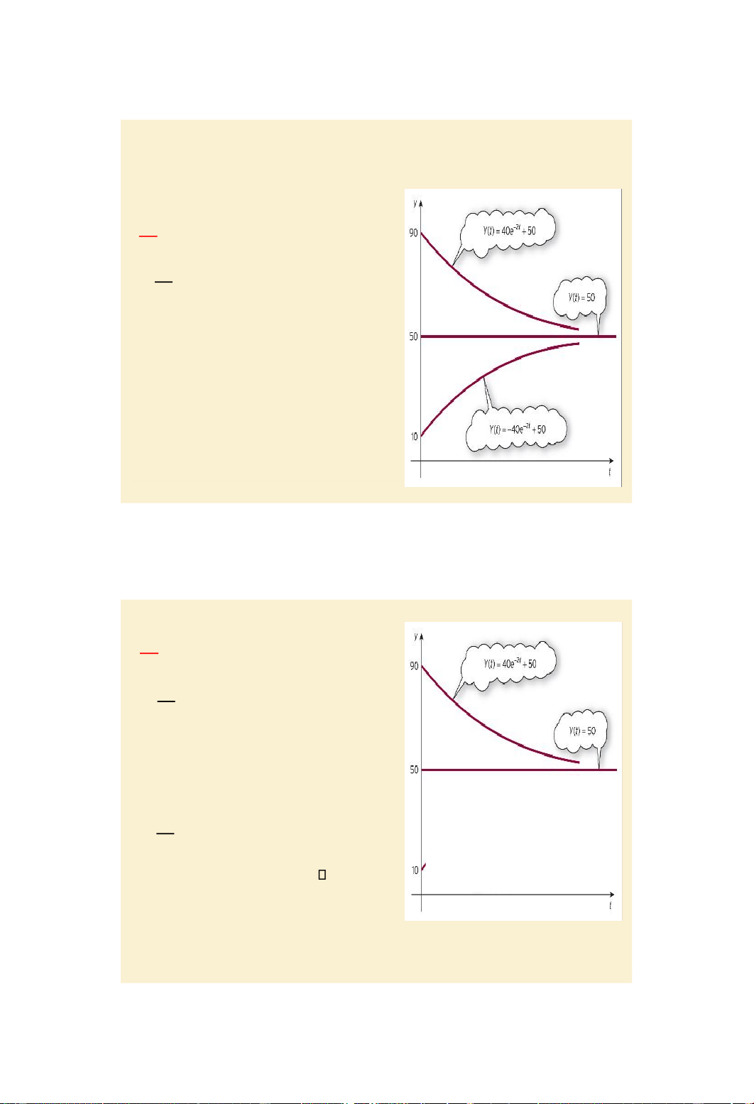
The graph (also cal ed time path) of y(t)
is the one at the bottom in figure 9.3a
converging to equilibrium value 50 (since m = -2 < 0). Figure 9.3 a
Jacques, Mathematics for Economics and Business, 7th edition ' Pearson Education Limited 2012 Slide 9.6
Solution of differential equation:
𝐝𝐲 = my + c with y(0)= y 𝐝𝐭 0 Example, page 645: b dy . = -2y + 100 with y(0) = 90. dt
Applying the 4-step solution procedure
we have the solution y(t) = 40e -2 t + 50.
The graph or time path of y(t) is the one
at the top in figure 9.3 converging to
equilibrium value 50 (since m = -2 < 0). c dy . = -2y + 100 with y(0) = 50. dt
Applying the 4-step solution procedure
we have the solution y(t) = 0 e -2 t + 50.
The graph or time path of y(t) = 50 is
the horizontal line in figure 9.3. Practice problem, page 648. Figure 9.3 b and c
Jacques, Mathematics for Economics and Business , 7 th edition ' Pearson Education Limited 2012 4 7/30/2020 lOMoAR cPSD| 47207194 Slide 9.7
Classifying solutions of differential equations: 𝐝𝐲
𝐝𝐭 = my + c with y(0)= y0 and analyzing stability of the economic model
General solution Value of A to satisfy y(0) = y0
m 0 y(t) = Aemt - c/m A = y0 + c/m m = 0 y(t) = A + ct A = y0 y(t) displays The model is m < 0 convergence stable Slide 9.8
National income determination
Recal that in Chapter 1, section 1.7, we learned about the simple two-sector macro-
economic model with structural equations: Y = C + I C = aY + b I = I*.
In practice, equilibrium balance Y = C + I (that means: the flow of money from firms
to households given as payment for the factors of production = the total flow of
money received by firms in form of investment or as payment for goods bought by
households) is not immediately attained. Instead of this equation, at any time
period, we assume that the rate of change of Y is proportional to the excess
expenditure. We can rewrite the above 03 equations as follows in the form of
timedependent equations (Y, C, I are functions of t): 𝐝𝐘
= 𝛂 𝐂 + 𝐈 − 𝐘 𝐝𝐭
(α is some positive adjustment coefficient, page 649) C = aY + b I = I*.
On substituting the expressions for C and I in the 1st equation, we have the
following (1st order linear) differential equation:
𝐝𝐘 = 𝛂 𝐚 − 𝟏)𝐘 + 𝛂(𝐛 + 𝐈∗. 𝐝𝐭
Jacques, Mathematics for Economics and Business , 7 th edition ' Pearson Education Limited 2012 5 7/30/2020 lOMoAR cPSD| 47207194 m > 0 divergence unstable
Jacques, Mathematics for Economics and Business, 7th edition ' Pearson Education Limited 2012
Jacques, Mathematics for Economics and Business , 7 th edition ' Pearson Education Limited 2012 6 7/30/2020 lOMoAR cPSD| 47207194 Slide 9.9
National income determination Example, page 650:
Consider a two-sector model 𝐝𝐘
= 𝟎. 𝟓 𝐂 + 𝐈 − 𝐘 𝐝𝐭 C = 0.8Y + 400 I = 600.
Find an expression for Y(t) when Y(0) = 7000. Is the system stable?
On substituting the expressions for C and I in the 1st equation, we
have the following (1st order linear) differential equation:
dY(t)/dt = -0.1Y + 500 with the initial condition Y(0) = 7000.
Applying the 4-step solution procedure we can derive the solution: Y(t) = 2000 e-0.1t +5000.
As t increases, e-0.1t converges to 0, and hence Y(t) converges to
the equilibrium level 5000. The time path displays convergence.
The given system / economic model is stable. Practice problem, page 651.
Jacques, Mathematics for Economics and Business, 7th edition ' Pearson Education Limited 2012 Slide 9.10
Supply and demand analysis
Recall that in Chapter 1, section 1.5, we learned about the singlecommodity
market model with structural equations: QS = aP - b QD = -cP + d QD = QS.
In practice, instead of assuming that QD = QS is immediately attained it is
more reasonable to assume the rate of change of price is proportional dP
to excess demand QD - QS , that is dt = α QD − QS, where α is some
positive adjustment coefficient (page 573). We can rewrite the above 03
equations as fol ows in the form of time – dependent supply and demand equations:
QS = aP - b QD = -cP + d dP = α QD − QS. dt
On substituting the expression of QS and QD into the 3rd equation,
we get: dP = −α a + c)P + α(d + b. dt
Jacques, Mathematics for Economics and Business , 7 th edition ' Pearson Education Limited 2012 7 7/30/2020 lOMoAR cPSD| 47207194 Slide 9.11
Supply and demand analysis Example, page 652: Consider the market model QS = 3P - 4 QD = -5P + 20 dPdt = 0.2 QD − QS .
Find expressions for P(t), QS(t) and QD(t). Is the system stable?
It is easy to get the following (1st order linear) differential equation: dP = -1.6P + 4.8. dt
with the initial condition P(0) = 2.
Applying the 4-step solution procedure we can derive the solution:
P(t) = -e-1.6t + 3, QS(t) = -3e-1.6t + 5 and QD(t) = 5e-1.6t + 5,
As t increases, e-1.6t converges to 0, and hence P(t), QS(t) and
QD(t) converge to the equilibrium levels of 3, 5 and 5, respectively. The system is stable. Slide 9.12
Supply and demand analysis Practice problem, page 653. Consider the market model QS = 2P - 2 QD = -P + 4 dP = 1 QD − QS. dt 3
Find expressions for P(t), QS(t) and QD(t) given P(0) = 1. Is the system stable? Key terms: page 653;
Exercise 9.2: problems 2, 4, 6, page 654;
Exercise 9.2*: problems 2, 5, pages 655 - 656.
Jacques, Mathematics for Economics and Business , 7 th edition ' Pearson Education Limited 2012 8 7/30/2020 lOMoAR cPSD| 47207194
Jacques, Mathematics for Economics and Business, 7th edition ' Pearson Education Limited 2012
Jacques, Mathematics for Economics and Business , 7 th edition ' Pearson Education Limited 2012 9 7/30/2020 lOMoAR cPSD| 47207194 Slide 9.13 Code A
Consider the supply and demand equations: QSt = 0.4Pt-1 - 15 QDt = - 0.8Pt + 30
Assuming that the equilibrium conditions prevail, find an
expression for Pt and Qt when P0 = 80. Is this system stable or unstable? Code B
Consider the two-sector model: dY/dt = 0.5(C + I* – Y) C = 0.6Y + 600 I* = 600
Find expressions for Y(t) when Y(0) = 2000. Is this system stable or unstable?
Jacques, Mathematics for Economics and Business, 7th edition ' Pearson Education Limited 2012 Slide 9.14
MAT1092: Quiz, time allowed 25’ Code A: Consider the market model QS = 4P - 1 QD = - 2P + 9 dP = 0.5 QD − QS . dt
Find expressions for P(t), QS(t) and QD(t) given P(0) = 1. Is the system stable? Code B: Consider a two-sector model Yt = Ct + It Ct = 0.6Yt-1 + 300 It = 0.2Yt-1 + 100.
Find an expression for Yt when Y0 = 3000. Is the system stable?
Jacques, Mathematics for Economics and Business , 7 th edition ' Pearson Education Limited 2012 10 7/30/2020 lOMoAR cPSD| 47207194 Slide 9.15
MAT1092: Quiz, time allowed 25’ Code A: Consider the market model QS = 3P - 2 QD = - 3P + 8 dPdt = 0.5 QD − QS .
Find expressions for P(t), QS(t) and QD(t) given P(0) = 1. Is the system stable? Code B: Consider a two-sector model Yt = Ct + It Ct = 0.5Yt-1 + 200 It = 0.3Yt-1 + 200.
Find an expression for Yt when Y0 = 3000. Is the system stable?
Jacques, Mathematics for Economics and Business, 7th edition ' Pearson Education Limited 2012 11