Chương 1: Economic Applications of Functions of One Variable | Môn toán cao cấp

lOMoAR cPSD| 49519085
Department of Mathematics, Faculty of Basic
Science, Foreign Trade University
-------------------------------------------------------------------------------------
Part 2, Analysis Chapter 1:
Economic Applications of Functions of One Variable
Instructor Dr. Son Lam CONTENTS lOMoAR cPSD| 49519085
II – The Application of derivatives in economics
---------------------------------------------------------------------------------------------------------------------------
I – Present and Future Value of Money
II – Application of Dirivatives in Economics
III – Economical optimization Definition lOMoAR cPSD| 49519085
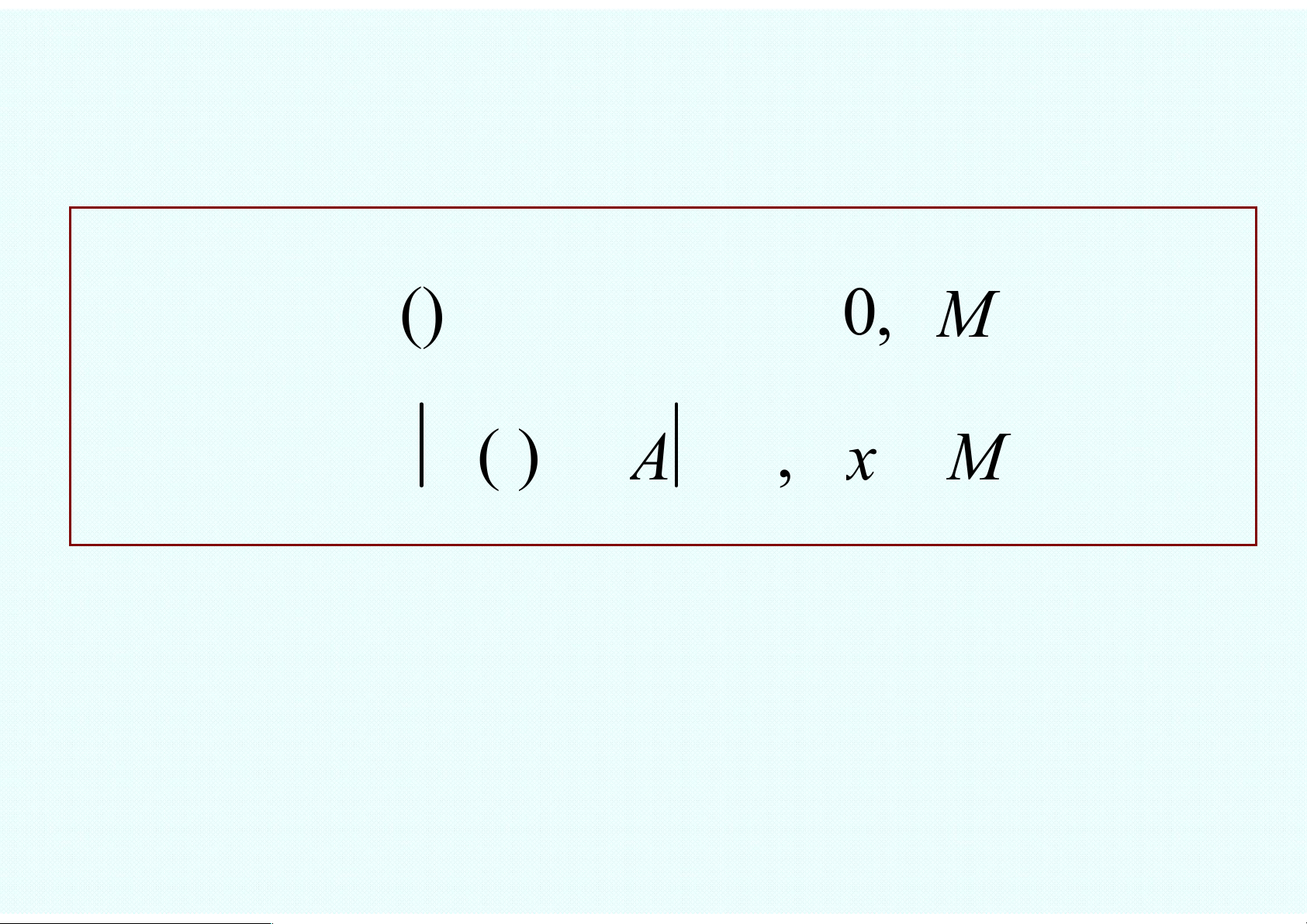
lim f x( ) = A⇔∀ε> ∃δ0, > 0 x→x0
satisfy: f x( ) − <A ε ∀ ∈, x (x0 −δ,x0 +δ) lOMoAR cPSD| 49519085
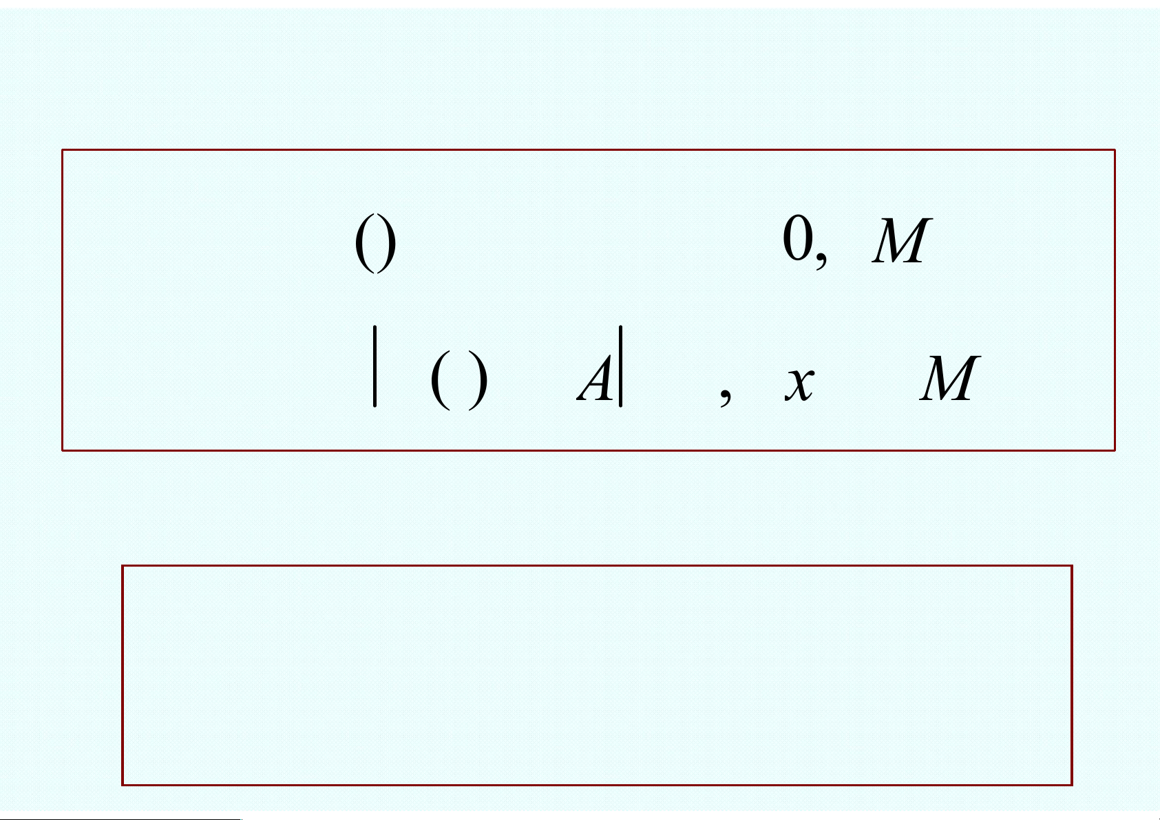
II – The Application of derivatives in economics Definition
lim f x( ) = A⇔∀ε> ∃δ0, > 0 x→x0
satisfy: f x( ) − <A ε ∀ ∈, x (x0 −δ,x0 +δ) lOMoAR cPSD| 49519085
II – The Application of derivatives in economics Definition lim () fx = > A ⇔∀ε>∃ M 0, 0 x→+∞ satisfy: ( ) f x − A <ε ∀ x > M , lOMoAR cPSD| 49519085
II – The Application of derivatives in economics lim () fx = > A ⇔∀ε>∃ M 0, 0 x→−∞ satisfy: ( ) f x − A x <ε ∀ <− M , Definition
lim f x( ) =+∞⇔∀ > ∃δM 0, > 0 x→x0
satisfy: f x( ) > M,∀ ∈x(x0 −δ,x0 +δ) lOMoAR cPSD| 49519085
II – The Application of derivatives in economics
lim f x( ) =−∞⇔∀ > ∃δM 0, > 0 x→x0
satisfy: f x( ) <−M,∀ ∈x (x0 −δ,x0 +δ) Definition lOMoAR cPSD| 49519085
II – The Application of derivatives in economics
lim f x( ) = A⇔∀{x }
n satisfy lim xn = x0 x x→ 0 n→+∞
then lim f x( n) = A n→+∞ Definition lOMoAR cPSD| 49519085
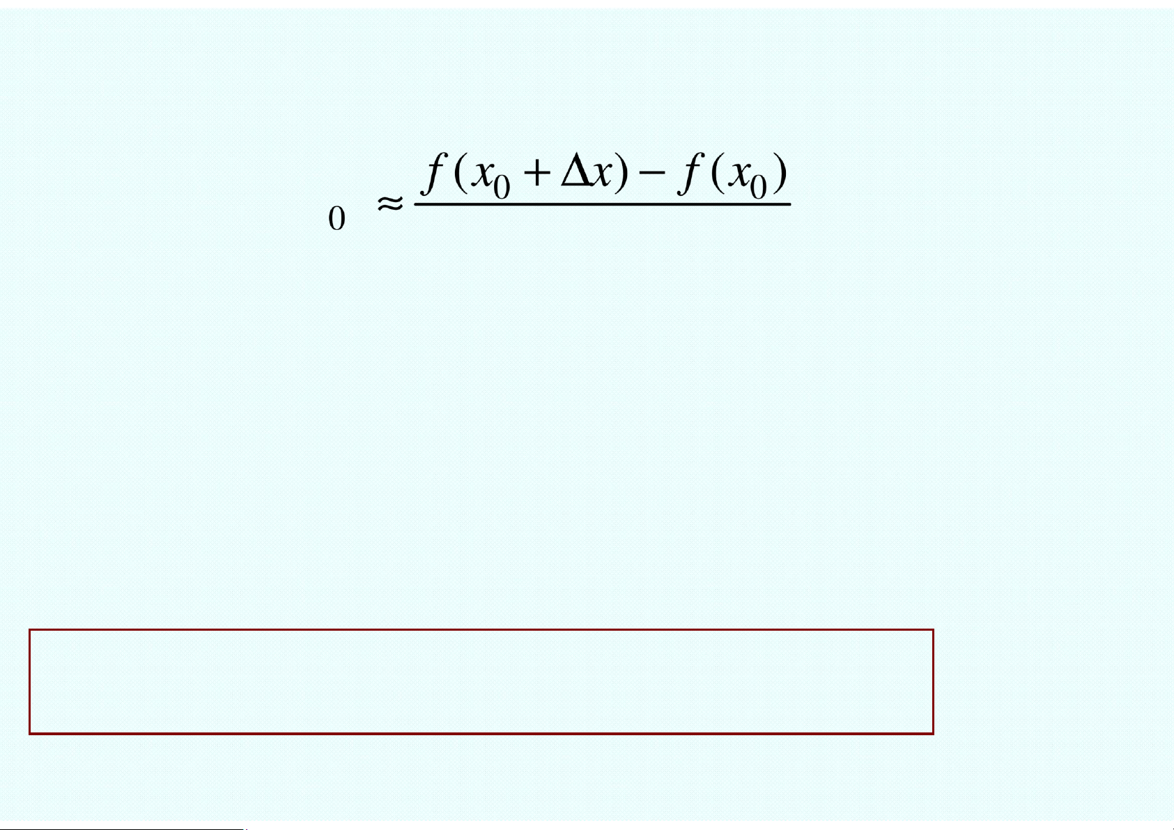
II – The Application of derivatives in economics f x( ) − f x( f ′(x0) = lim 0) x x→ x − x 0 0
= lim 0 x) − f x( 0) f x( + ∆ ∆ →x 0 ∆x Example lOMoAR cPSD| 49519085
II – The Application of derivatives in economics
f x( )=3x2, f’(2)= ? 2 −12 f x( )− f (2) 3x f ′(2) = lim = lim = lim 3x( +6) =12
x→2 x −2 x→2 x −2 x→2 f x( )− f x( f ′(x0) = lim
0) = lim 3x2 −3x02 = lim 3x( +3x0) = 6x0 x − x x x→ 0 0
x→2 x − x0 x→2 lOMoAR cPSD| 49519085
II – The Application of derivatives in economics (3x2)' = 6x Example
g x( ) = x g, '( )0 = ? Application lOMoAR cPSD| 49519085
II – The Application of derivatives in economics f ′( )x ∆x
f x( 0 + ∆x) − f x( 0) ≈ f ′(x0).∆x
f x( 0 +1) − f x( )0 ≈ f ′( )x0 lOMoAR cPSD| 49519085
II – The Application of derivatives in economics Concept
Considering the economic function y = f(x) representing
the effect of the economic variable x on the economic variable y.
My x( )0 = f ′( )x0
is called the y-marginal value of x at the point x0.
Meaning: at the point x0, if x increases by 1 unit, then y
changes by an amount approximately equal to units ′ f ( )x0 lOMoAR cPSD| 49519085
II – The Application of derivatives in economics Example
Marginal Quantitives = Marginal Physical Product
Q = f L( ) MPPL = f ′( )L
Q = g K( ) MPPK = g K′( ) lOMoAR cPSD| 49519085
II – The Application of derivatives in economics
Marginal Revenue TR TRQ= ( ) MR TR Q=′( )
Marginal Cost TC TC Q= ( ) MC TC Q= ′( )
Marginal Propensity to C CY= ( ) MPC C Y= ′( ) Consume Concept lOMoAR cPSD| 49519085
From a mathematical perspective, for the function y
= f(x) to obey the law of diminishing marginal utility, then
f ′′( ) 0x < When x is large enough. Example:
Detemine the condition for the function to obey the law of diminishing marginal utility
Q = aL , aα >0,α>0,L >0 lOMoAR cPSD| 49519085
II – The Application of derivatives in economics Concept
Considering the economic function y = f(x) representing the
effect of the economic variable x on the economic variable y.
εx oy(x ) = y x′( o).xo y x( 0)
Is called the elasticity of y with respect to x at the point x0.
Meaning: at the point x0, if x increases by 1%, then y
changes by an amount approximately equal to ε (%) lOMoAR cPSD| 49519085
II – The Application of derivatives in economics
Example: Calculate the price elasticity of demand at p0=4$
given D= −6p p2 Example
Calculate the price elasticity of demand at p0=4$ given
demand function: D= −6p p2 Condition :0 < p < 6 lOMoAR cPSD| 49519085
II – The Application of derivatives in economics εQp = D (p)D(p)′ .p = 66p−2p2 .p εpD (4) = −82.4 =−1( )% −p •Meaning:
•At the price po = 4, if the price increases by 1%, the demand will
decrease by approximately 1%. •If the price increases by 2%, the
demand will decrease by an amount of approximately 2*1% = 2%.
•If the price increases by 3.2%, the demand will decrease by approximately 3.2*1% = 3.2%. Example lOMoAR cPSD| 49519085
II – The Application of derivatives in economics
Calculate the labor elasticity of output, given demand function:
Q = aL , aα >0,α>0,L >0 α−1 εLQ( L ) = Q'( L ).L =α aLα L =α Q( L ) aL •Meaning: