Chương 11 : Differentiation | Môn toán cao cấp
From a strictly commercial perspective, the ideal regulations would maximize the number of fish available for the year-to-year fish harvest. The key to finding those ideal regulations is a mathematical function called the reproduction curve. For a given fish habitat, this function estimates the fish population a year from now, P(n +1), based. Tài liệu giúp bạn tham khảo, ôn tập và đạt kết quả cao. Mời bạn đọc đón xem !
Môn: Toán Cao Cấp (KTHCM) 189 tài liệu
Trường: Đại học Kinh tế Thành phố Hồ Chí Minh 2.1 K tài liệu
Tác giả:


Preview text:
lOMoAR cPSD| 49519085 11.1 The Derivative
commercial fishing boats in a season. This prevents overfishing, which depletes the
fish population and leaves, in the long run, fewer fish to catch. 11.2 Rules for Differentiation
From a strictly commercial perspective, the ideal regulations would maximize the 11.3 The Derivative as a
number of fish available for the year-to-year fish harvest. The key to finding those Rate of Change
ideal regulations is a mathematical function called the reproduction curve. For a given
fish habitat, this function estimates the fish population a year from now, P(n +1), based 11.4 The Product Rule and the Quotient Rule
on the population now, P(n)
, assuming no external interventions such as fishing or influx of predators. 11.5 The Chain Rule Chapter
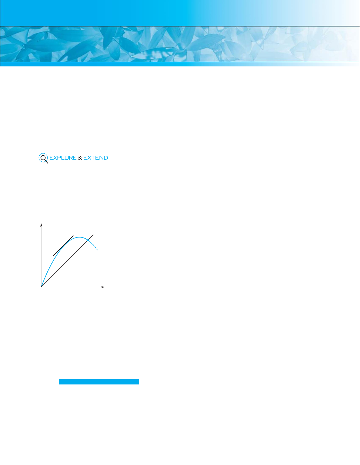
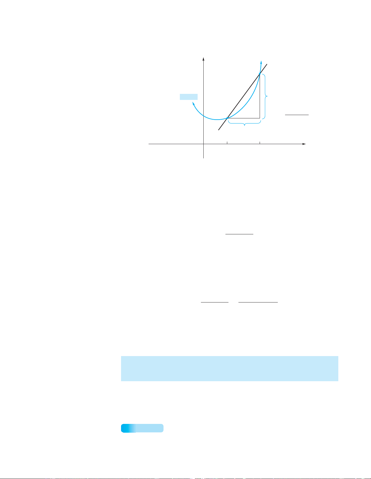
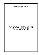
Thefiguretothebottomleftshowsatypicalreproductioncurve.Alsographedisthe line 11 Review
P(n+1) = P(n), the line along which the populations P(n+1) and P(n) would be equal.
Notice the intersection of the curve and the straight line at point A.This is where,
because of habitat crowding, the population has reached its maximum sustainable size. Marginal Propensity
A population that is this size one year will be the same size the next year. to Consume
For any point on the horizontal axis, the distance between the reproduction curve
and the line P(n + 1) = P(n) represents the sustainable harvest: the number of fish that
could be caught, after the spawn have grown to maturity, so that in the end the
population is back at the same size it was a year ago.
Commercially speaking, the optimal population size is the one where the distance P ( n
between the reproduction curve and the line P(n + 1) = P(n) is the greatest. This 1)
condition is met where the slopes of the reproduction curve and the line P(n + 1) =
P(n) are equal. [The slope of P(n + 1) = P(n) is, of course, 1.] Thus, for a maximum A
fish harvest year after year, regulations should aim to keep the fish population fairly close to P0.
A central idea here is that of the slope of a curve at a given point. That idea is the
cornerstone concept of this chapter.
Now we begin our study of calculus. The ideas involved in calculus are completely P ( n )
different from those of algebra and geometry. The power and importance of these ideas P 0 and their G overnment 11 Differentiation
regulations generally limit the
applications will become clear later in the book. In this chapter we introduce the number of fish taken from a
derivative of a function and the important rules for finding derivatives. We also show given fishing ground by 495 lOMoAR cPSD| 49519085 496 Chapter 11 Differentiation how the derivative is used to
quantity, such as the rate at which the position of a body is changing.
analyze the rate of change of a
From Introductory Mathematical Analysis For Business, Economics, and the Life and Social Sciences, Thirteenth Edition.
Ernest F. Haeussler, Jr., Richard S. Paul, Richard J.Wood. Copyright © 2011 by Pearson Education, Inc. All rights reserved. Objective 11.1 The Derivative
To develop the idea of a tangent line
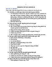
The main problem of differential calculus deals with finding the slope of the tangent
to a curve, to de ne the slope of a
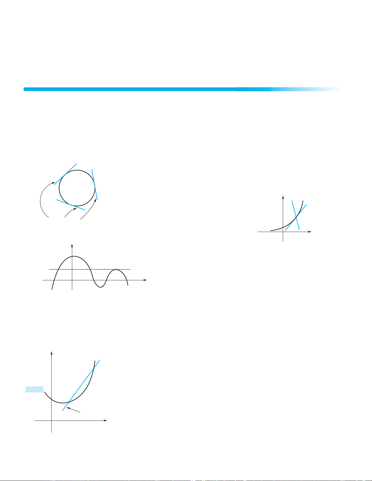
line at a point on a curve. In high school geometry a tangent line, or tangent, to a circle
curve, and to de ne a derivative and
is often defined as a line that meets the circle at exactly one point (Figure 11.1).
give it a geometric interpretation. To
compute derivatives by using the limit However, this idea of a tangent is not very useful for other kinds of curves. For de nition.
example, in Figure 11.2(a), the lines L1 and L2 intersect the curve at exactly one point
P. Although we would not think of L2 as the tangent at this point, it seems natural that L1 is. In
Figure 11.2(b) we intuitively would consider L3 to be the tangent at point P, even though L3
intersects the curve at other points. y y L 2 L 1 P Tangent lines
FIGURE11.1 Tangentlinesto a circle. P L 3 x x L1 is a tangent line
L3 is a tangent at P, but L2 is not. line at P. (a) (b) FIGURE 11.2 Tangent line at a point.
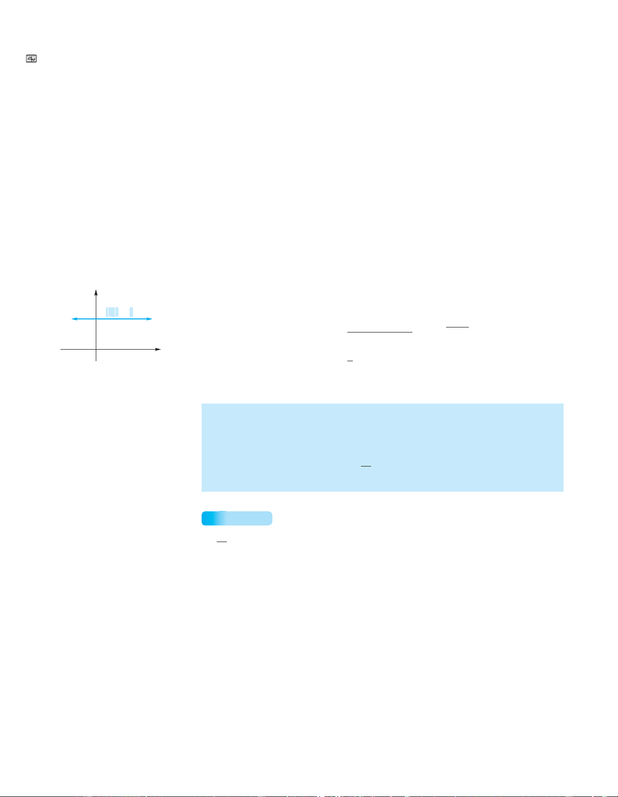
Fromtheseexamples,weseethattheideaofatangentassimplyalinethatintersects
y a curve at only one point is inadequate. To obtain a suitable definition of tangent line,
we use the limit concept and the geometric notion of a secant line. A secant line is a
line that intersects a curve at two or more points. Q
Look at the graph of the function y = f (x) in Figure 11.3. We wish to define the
tangent line at point P. If Q is a different point on the curve, the line PQ is a secant line.
If Q moves along the curve and approaches P from the right (see Figure 11.4), typical
y f ( x )
secant lines are PQ, PQ, and so on. As Q approaches P from the left, typical secant lines P
are PQ1, PQ2, and so on. In both cases, the secant lines approach the same limiting
position. This common limiting position of the secant lines is defined to be the tangent Secant line
line to the curve at P. This definition seems reasonable and applies to curves in general, x not just circles. lOMoAR cPSD| 49519085 Section 11.1 The Derivative A
FIGURE 11.3 Secant line PQ.
the curveline through (0,0) and a nearby point to its right on the curve must always be
the liney = |x| does not have a tangent at (0,0).As can be seen in Figure 11.5, a secant y
curve does not necessarily have a tangent line at each of its points. For example, y y x
y x , x 0 y x, x 0 x (0 , 0)
FIGURE 11.5 No tangent line to
FIGURE 11.4 The tangent line is a limiting position of secant lines.
graph of y = |x| at (0,0). PQ Q PQ PQ PQ 496 PQ 1 PQ 2 493 P PQ 3 Limiting position (t angent at P )
y = x. Thus the limiting position of such secant
lines is also the line y x = x. However, a secant
line through (0,0) and a nearby point to its left
on the curve must always be the line y = −x. Hence, the limiting position of such secant
lines is also the line y = −x. Since there is no common limiting position, there is no tangent line at (0,0).
Now that we have a suitable definition of a tangent to a curve at a point, we can
define the slope of a curve at a point. Definition
The slope of a curve at a point P is the slope, if it exists, of the tangent line at P.
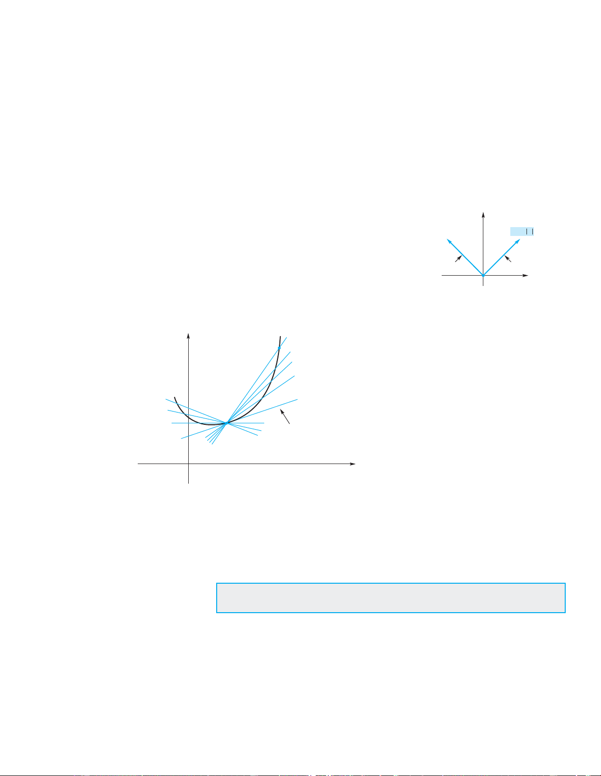
Since the tangent at P is a limiting position of secant lines PQ, we consider the
slope of the tangent to be the limiting value of the slopes of the secant lines as Q
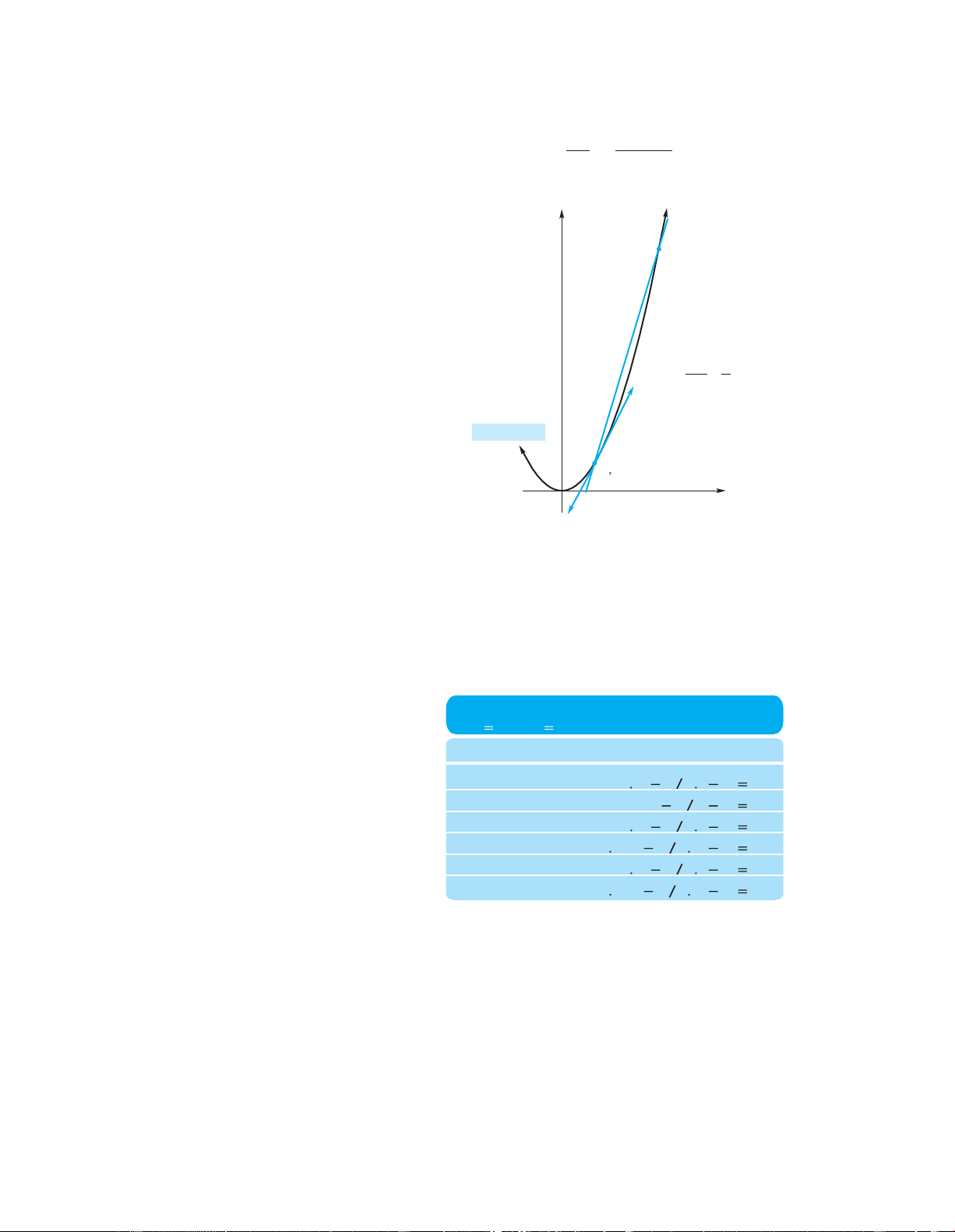
approaches P. For example, let us consider the curve f (x) = x2 and the slopes of some
secant lines PQ, where P = (1,1). For the point Q = (2.5,6.25), the slope of PQ (see Figure 11.6) is 497 lOMoAR cPSD| 49519085 498 Chapter 11 Differentiation = rise = 6.25−− 1 = mPQ 3.5 run 2.5 1 y Q (2.5 , 6.25) m 6.25 PQ 1 2.5 1 3.5
y f ( x ) x 2 Tangent line P (1, 1) x
FIGURE 11.6 Secant line to f (x) = x2 through (1, 1) and (2.5, 6.25).
Table 11.1 includes other points Q on the curve, as well as the corresponding
slopes of PQ. Notice that as Q approaches P, the slopes of the secant lines seem to
approach 2. Thus, we expect the slope of the indicated tangent line at (1, 1) to be 2.
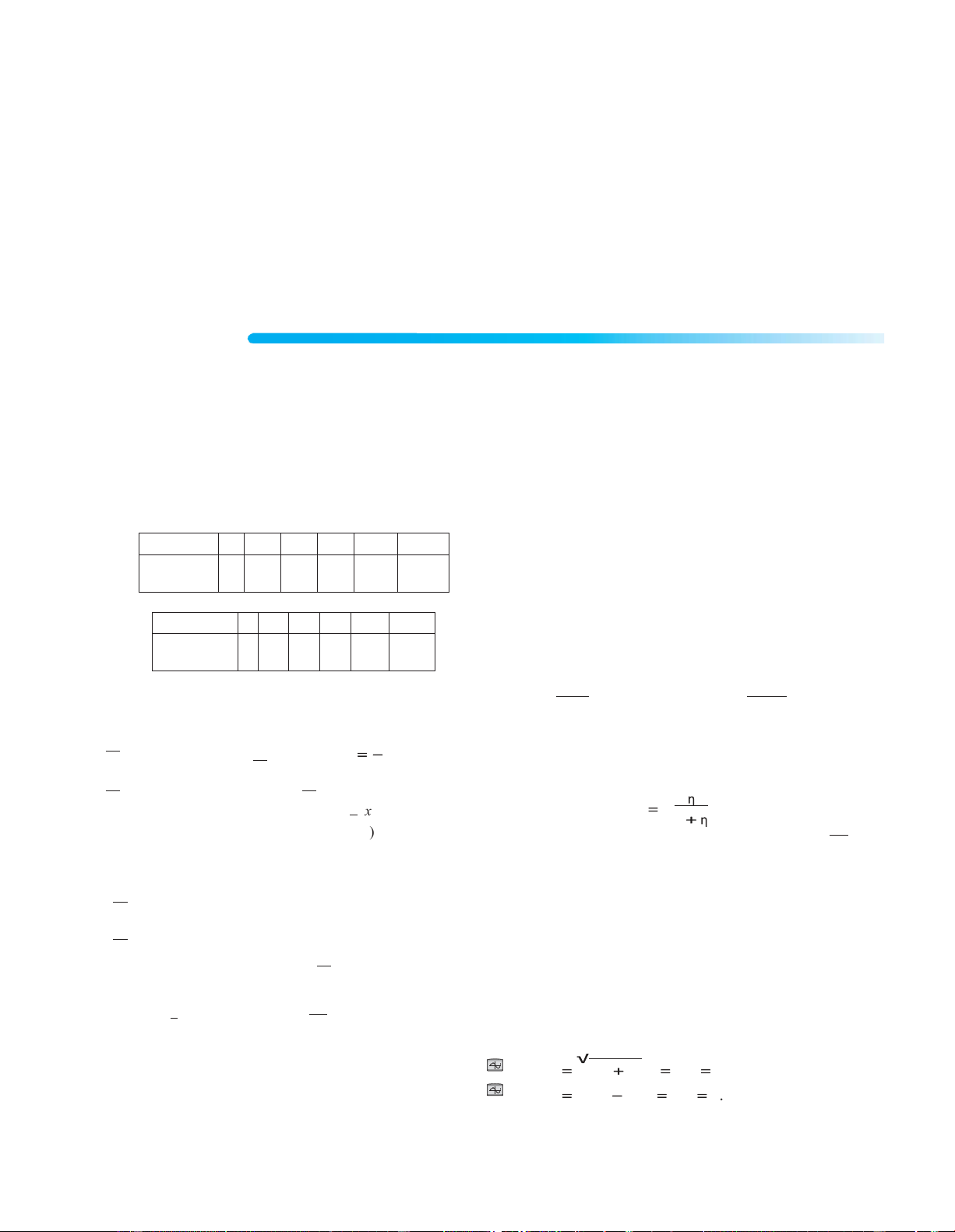
This will be confirmed later, in Example 1. But first, we wish to generalize our procedure. Table11.1
SlopesofSecantLinestotheCurve
f ( x ) x 2 at P (1 , 1) Q Slopeof PQ (2.5,6.25) (6 25 1) (2 5 1) 3.5 (2 , 4) (4 1) (2 1) 3 (1.5,2.25) (2 25 1) (1 5 1) 2.5 (1.25,1.5625) (1 5625 1) (1 25 1) 2.25 (1.1,1.21) (1 21 1) (1 1 1) 2.1 (1.01,1.0201) (1 0201 1) (1 01 1) 2.01 lOMoAR cPSD| 49519085 Section 11.1 The Derivative y Q
( z , f ( z ))
y f ( x )
f ( z ) f ( a )
( a , f ( a )) f ( z ) m f ( a ) PQ z a
P z a h x a z
FIGURE 11.7 Secant line through P and Q.
the pointFor the curveP = (a,fy(a=)). Iff (xQ) in Figure 11.7, we will find an expression for
the slope at= (z,f (z)), the slope of the secant line PQ is f (z) mPQ =
z −− fa(a)
h = If the difference0, for if h = 0, thenz − az is called= a, and no secant line exists.
Accordingly,h, then we can write z as a + h. Here we must have m =
PQ f (zz) −− fa(a) = f (a + hh) − f (a)
Which of these two forms for mPQ is most convenient depends on the nature of the
function f . As Q moves along the curve toward P, z approaches a. This means that h
approaches zero. The limiting value of the slopes of the secant lines—which is the
slope of the tangent line at (a,f (a))—is
f (z) f (a)
f (a h) f (a)
mtan = lim − = lim + − z→a z − a h→0 h (1)
Again, which of these two forms is most convenient—which limit is easiest to
determine—depends on the nature of the function f . In Example 1, we will use this
limit to confirm our previous expectation that the slope of the tangent line to the curve
f (x) = x2 at (1, 1) is 2.
EXAMPLE 1 Finding the Slope of a Tangent Line 499 lOMoAR cPSD| 49519085 500 Chapter 11 Differentiation
Find the slope of the tangent line to the curve y = f (x) = x2 at the point (1, 1).
Solution: The slope is the limit in Equation (1) with f (x) = x2 and a = 1:
hlim→0 f (1 + hh) − f (1) = hlim→0 (1 + h)h2 − (1)2
h→0 1 + 2h +h h2 − 1 = hlim→0 2h +h h2 = lim h(2
= hlim→0 h+ h) = hlim→0 (2 + h) = 2
Therefore, the tangent line to y = x2 at (1, 1) has slope 2. (Refer to Figure 11.6.) Now Work Problem 1 498
Calculating a derivative via the definition 495
We can generalize Equation (1) so that it applies to any point (x,f (x)) on a curve.
Replacing a by x gives a function, called the derivative of f , whose input is x and
whose output is the slope of the tangent line to the curve at (x,f (x)), provided that the
tangent line exists and has a slope. (If the tangent line exists but is vertical, then it has
no slope.) We thus have the following definition, which forms the basis of differential calculus: Definition
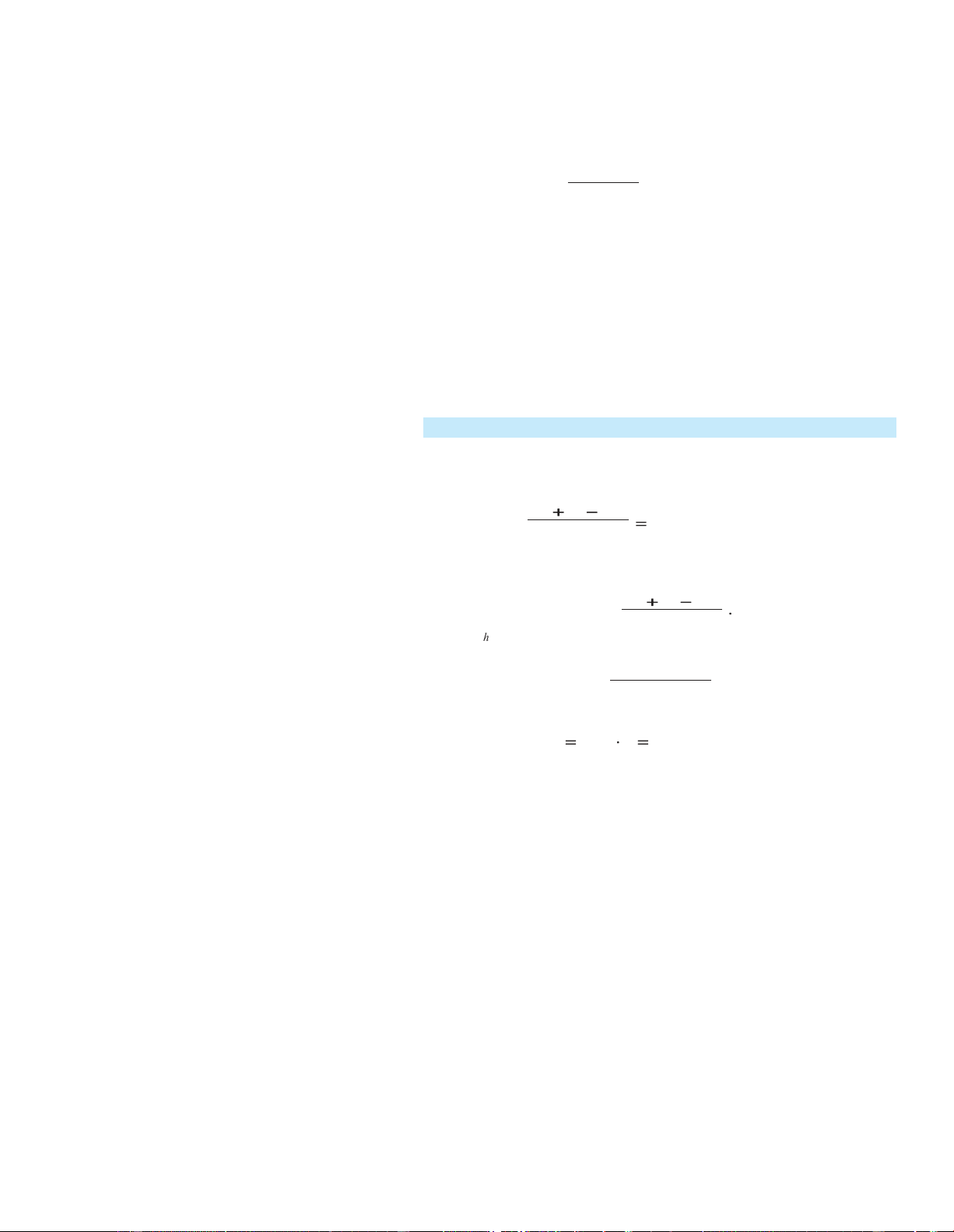
The derivative of a function f is the function denoted f (read “f prime”) and defined by
f (z) f (x)
f (x h) f (x) f (x) = lim −− = lim + −
(2) z→x z x h→0 h
provided that this limit exists. If f (a) can be found [while perhaps not all f (x) can
be found] f is said to be differentiable at a, and f (a) is called the derivative of f at
a or the derivative of f with respect to x at a. The process of finding the derivative
is called differentiation.
In the definition of the derivative, the expression
f (z) −− f (x) = f (x + h) − f (x) z x h lOMoAR cPSD| 49519085 Section 11.1 The Derivative
where z = x + h, is called a difference quotient. Thus f (x) is the limit of a difference quotient. EXAMPLE 2
Using the Definition to Find the Derivative
If f (x) = x2, find the derivative of f .
Solution: Applying the definition of a derivative gives
difference quotient requires considerable
f (x) = hlim→0 + hh) − f (x) f
manipulation before the limit step is (x
taken. This requires that each written
step be preceded by “limh→0” to
= hlim→0 (x + hh)2 − x2 = hlim→0 x2 + 2xhh+ h2 − x2
acknowledge that the limit step is still
pending. Observe that after the limit step
is taken, h will no longer be present.
= hlim→0 2xhh+ h2 = hlim→0 h(2xh+ h) = hlim→0 (2x + h) = 2x
Observe that, in taking the limit, we treated x as a constant, because it was h, not x,
that was changing.Also, note thatas giving the slope of the tangent line to the graph
off (x) = 2x defines a function off at (xx, which we can interpret,f (x)). For example, if
x = 1, then the slope is f (1) = 2 · 1 = 2, which confirms the result in Example 1. Now Work Problem 3
Besides the notation f (x), other common ways to denote the derivative of y = f (x) CAUTION at x are
requires precision. Typically, the 501 lOMoAR cPSD| 49519085 502 Chapter 11 Differentiation dy dy
The notation , which is called Leibniz dx
notation, should not be thought of as a fraction, although dx
pronounced “dee y,dee x” or “dee y by dee x”
it looks like one. It is a single symbol for a derivative.
We have not yet attached any meaning to individual d
symbols such as dy and dx. ( f (x))
“dee f (x),dee x” or “dee by dee x of f (x)” dx y “y prime” Dxy
“dee x of y” Because the
Dx( f (x))
“dee x of f (x)”
derivative gives the slope of the tangent line, f (a) is the slope of the line tangent to
the graph of y = f (x) at (a,f (a)).
Two other notations for the derivative of f at a are dy and y(a) dx x=a
EXAMPLE 3 Finding an Equation of a Tangent Line
If f (x) = 2x2 + 2x + 3, find an equation of the tangent line to the graph of f at (1,7). Solution:
Strategy We will first determine the slope of the tangent line by computing the point-
slope form gives an equation of the tangent line.derivative and evaluating it at x = 1.
Using this result and the point (1,7) in a We have
The derivative must beIn Example 3 it issince the derivative is 4not correct to say that,x +x +2, the tangent2)(xat the− 1).) f (x)
= hhlimlim→0 f2(2((xx2x+++h4hh)xh)−2 ++f (22(xh)x2 ++h2)x++3)2h−+(23x−2 +2x22x−+23)x − 3 line at (1,7) is y − 7 = (4 = →0 h
(This is not even the equation of a line. evaluated lim =
point of tangency to determine the slope h→0 h of the tangent line.
4 xh 2 h 2 2 h lOMoAR cPSD| 49519085 Section 11.1 The Derivative = hlim→0 h
= hlim→0 (4x + 2h + 2) So
f (x) = 4x + 2 and f (1) = 4(1) + 2 = 6
Thus, the tangent line to the graph at (1, 7) has slope 6. A point-slope form of this tangent is
y − 7 = 6(x − 1)
which in slope-intercept form is y = 6x + 1 Now Work Problem 25
EXAMPLE 4 Finding the Slope of a Curve at a Point Find
the slope of the curve y = 2x + 3 at the point where x = 6.
2Solution:x + 3, we haveThe slope of the curve is the slope of the tangent line. Lettingdxdy → f
(x + h) − f (x) = hlim→0 (2(x + h) + h3) − (2x + 3) y = f (x) = lim h 0 h 2 h lim 2 = hlim→0 h 0 h → 2
Since dy/dx = 2, the slope when x = 6, or in fact at any point, is 2. Note that the curve is
a straight line and thus has the same slope at each point. Now Work Problem 19
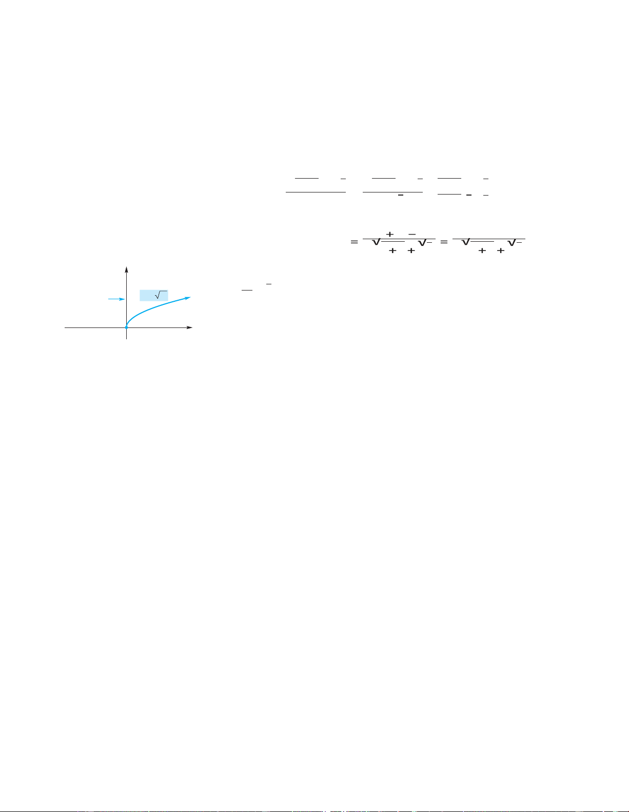
EXAMPLE 5 A Function with a Vertical Tangent Line Find d (√x). dx Solution:
Lettingd f (x) = √x, we have f ( x (
h ) f ( x ) x ) lim lim
√x + h − √x dx = h→0 h = h→0 h 500 503 lOMoAR cPSD| 49519085 504 Chapter 11 Differentiation Rationalizing numerators or
denominators of fractions is often
helpful in calculating limits. 497
As h → 0, both the numerator and denominator approach zero. This can be avoided by
rationalizing the numerator:
√x + h − √x = √x + hh − √x.√√xx ++ hh ++ √√xx h
( x h ) x h
h ( x h x )
h ( x h x ) y Tangent y line at x (0, 0) x
FIGURE11.8 Verticaltangent Therefore, = Now Work Problem 17
because the tangent line is vertical at that point. It is worthwhile to mention thatIn
Example 5 we saw that the function y = √x is not differentiable whenyx==|x0|, line at
all at that point. (Refer to Figure 11.5.) Both examples show that the domain ofalso is
not differentiable when x = 0, but for a different reason: There is no tangent f may be
strictly contained in the domain of f .
To indicate a derivative, Leibniz notation is often useful because it makes it con-
Variables other than x and y are often
venient to emphasize the independent and dependent variables involved. For example, lOMoAR cPSD| 49519085 Section 11.1 The Derivative
more natural in applied problems. Time
if the variable p is a function of the variable q, we speak of the derivative of p with
denoted by t, quantity by q, and price by
respect to q, written dp/dq.
p are obvious examples. Example 6 illustrates. d h 1 1 1 ( x ) lim lim dx
h 0 h ( x h x ) x h x x x 2 x Notethattheoriginalfunction,
x ,isdefinedfor x 0 ,butitsderivative, 1 (2 x ) ,
isdefinedonlywhen x 0 .Thereasonforthisisclearfromthegraphof y x in line at (0, 0). Figure 11.8. When x
0, the tangent is a vertical line, so its slope is not defined. APPLY IT
d f (q + h) − f (q) dq = dqh
1.Ifaballisthrownupwardataspeedof
40ft/s from a height of 6 feet, its height
H in feet after t seconds is given by 1 1
q − (q + h)
= + − 2. Find dH . H 6 40t 16t − 2q 2q(q dt EXAMPLE 6 Finding the
= hlim→0 2(q + hh) = hlim→0 h+ h)
Derivative of p with Respect to q 1 dp
= hlim→0 hq(2−q((qq++hh))) = hlim→0 h(2q(−qh+ h))
If p = f (q) = 2q, find dq. 1 1 lim
h 0 2 q ( q h ) 2 q 2
Solution:used so far) and then We also have
usingWe will do this problem first
using ther → q to illustrate the dq dp
other variant of the limit.h = rlim → 0
→q f (rr) −− qf (q) limit (the only one we have 1 1 q − r 1 2r − 2q 2rq 2 lim q h 0
= rlim→q r − q = rlim→q r − q d p
= rlim→q 2−rq1 = 2−q12
We leave it you to decide which form leads to the simpler limit calculation in this case.
Note that when q = 0 the function is not defined, so the derivative is also not even defined when q = 0. Now Work Problem 15
Keep in mind that the derivative of y = f (x) at x is nothing more than a limit, namely
f (x + h) − f (x) lim h→0 h 505 lOMoAR cPSD| 49519085 506 Chapter 11 Differentiation equivalently
f (z) − f (x) lim z→x z − x
whoseusewehavejustillustrated.Althoughwecaninterpretthederivativeasafunction that
gives the slope of the tangent line to the curve y = f (x) at the point (x,f (x)), this
interpretation is simply a geometric convenience that assists our understanding. The
preceding limit may exist, aside from any geometric considerations at all. As we will
see later, there are other useful interpretations of the derivative.
In Section 11.4, we will make technical use of the following relationship between
differentiability and continuity. However, it is of fundamental importance and needs
to be understood from the outset.
If f is differentiable at a, then f is continuous at a.
To establish this result, we will assume that f is differentiable at a.Then f (a) exists, and a f f ( h) (a) lim h 0 h f (a) →
Consider the numerator f (a + h) − f (a) as h → 0. We have
lim (f (a + h) − f (a)) = a h f ( h) lim f h 0 h ( a ) h→0 → =
f (a + h) − f (a) · lim lim h h→0 h h→0 f ( a ) 0 0
Thus, limh→0 (f (a + h) − f (a)) = 0. This means that f (a + h) − f (a) approaches 0 as lOMoAR cPSD| 49519085 Section 11.1 The Derivative y h → 0. Consequently,
lim f ( a h ) h 0 f (a) →
As stated in Section 10.3, this condition means that f is continuous at a. The foregoing, then, proves that f is continuous at
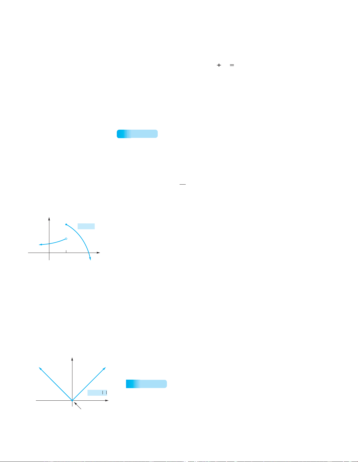
FIGURE 11.9 f is not continuous at
If a function is not continuous at a point, then it cannot have a derivative there.
a, so f is not differentiable at a.
For example, the function in Figure 11.9 is discontinuous at a. The curve has no
tangent at that point, so the function is not differentiable there. EXAMPLE 7
Continuity and Differentiability
a. Let f (x) = x2. The derivative, 2x, is defined for all values of x, so f (x) = x2 must be
continuous for all values of x. 1
b. The function f (p) =
is not continuous at p = 0 because f is not defined there. 2p
Thus, the derivative does not exist at p = 0.
a when f is differentiable there. More simply, we say that differentiability at a point
y f ( x )
implies continuity at that point. x a 502 499
y The converse of the statement that differentiability implies continuity is false. That is,
continuity does not imply differentiability. In Example 8, we give a function that is
continuous at a point, but not differentiable there.
EXAMPLE 8 Continuity Does Not Imply Differentiability
f ( x ) x
The function y = f (x) = |x| is continuous at x = 0. (See Figure 11.10.) As we
x mentioned earlier, there is no tangent line at x = 0. Thus, the derivative does not exist 507 lOMoAR cPSD| 49519085 508 Chapter 11 Differentiation
Continuous at x 0, but
there. This shows that continuity does not imply differentiability.
not differentiable at x 0
FIGURE 11.10 Continuity does not
imply differentiability. Finally, we remark that while differentiability of f at a implies continuity of f at a, the derivative function,
f , is not necessarily continuous at a. Unfortunately, the classic example is constructed
from a function not considered in this book. PROBLEMS 11.1
In Problems 1 and 2, a function f and a point P on its graph are
17. f ( x ) if f (x) = √2x 18. H(x) if H(x) = given. (a)
Find the slope of the secant line PQ for each point Q =
19. Find the slope of the curve y = x2 + 4 at the point (−2,8).
(x,f (x)) whose x-value is given in the table. Round your answers to four decimal places.
20. Find the slope of the curve y = 1 − x2 at the point (1,0). (b)
22.21. Find the slope of the curveFind the slope of the curve yy
Use your results from part (a) to estimate the slope of the tangent line at P.
== √4x22x−when5 whenx =x18.= 0.
1. f (x) = x3 + 3,P = (−2,−5)
x-value of Q −3 −2.5 −2.2 −2.1 −2.01 −2.001
In Problems 23–28, find an equation of the tangent line to the mPQ
curve at the given point. 2. 23. y
f (x) = ex, P = (0,1) = x + 4; (3, 7)
24. y = 3x2 − 4;(1,−1)
x-value of Q 1 0.5 0.2 0.1 0.01 0.001
25. y = x2 + 2x + 3;(1,6)
26. y = (x − 7)2; (6, 1) mPQ 4 5
In Problems 3–18, use the definition of the derivative to find each of the following. 27. y = x + 1; (3,1) 28. y = 1 − 3x;(2,−1) 3.) f ( if x
f (x) = x 4.)
if f (x) f = ( 4 x x − 1 dy dy 29. Banking
Equations may involve derivatives of
functions. In an article on interest rate deregulation, Christofi
5. if y = 3x + 5 6. if y 5
and Agapos1 solve the equation x dx dx dx d 1 dC 7. dx (3 − 2x) 8. − dx2 1 9. f (x)
10. f ( x if f (x) = 3) if
f (x) = 7.01 d r rL − dD 2 + − 12. y
if y = x2 + 3x + 2
for η (the Greek letter “eta”). Here r is the deposit rate paid by
commercial banks, rL is the rate earned by commercial banks, 11.(x 4x 8) dx
C is the administrative cost of transforming deposits into dp 2 d 2
return-earning assets, D is the savings deposits level, and η is
the deposit elasticity with respect to the deposit rate. Find η. 13. dq
p = q + q +
14. dx x − x − 6 dC
In Problems 30 and 31, use the numerical derivative feature of 2
your graphing calculator to estimate the derivatives of the 15. y 16. if y = x
if C = 7 + 2q − 3q
functions at the indicated values. Round your answers to three dq decimal places. 3 if 3 2 1 ( 3)
30. f ( x ) 2 x 2 3 x ; x 1 , x 2
31. f ( x ) e x (4 x 7) ; x 0 , x 1 5 lOMoAR cPSD| 49519085 Section 11.1 The Derivative
In Problems 32 and 33, use the “limit of a difference quotient”
A. Christofi and A. Agapos, “Interest Rate Deregulation: An Empirical
approach to estimate f (x) at the indicated values of x. Round
Justification,” Review of Business and Economic Research, XX, no. 1 (1984),
your answers to three decimal places. 39–49. x 2
32. f ( x ) x ln x x ; x 1 , x 10 x 2 4 x 2
33. f ( x ) ; x 2 , x 4 x 3 3 1
34.at the point (Find an equation of the tangent line to the curve−2,2). Graph both the curve and the tangent line.f (x) = x2 + x have positive
slopes over these intervals. Observe the intervalwherehave negative slopes over this interval.f (x) is negative. Notice that tangent lines to the graph of f
Notice that the tangent line is a good approximation to the curve
35. The derivative of f (x) = x − both the function f and its derivative points on the graph of f where the tangent line is horizontal.
36. n 4, n 3, n 2 ; f ( x ) if f ( x ) 2 x 4 x 3 3 x 2
37. n 5 , n ;
3 f ( x ) if f ( x ) 4 x 5 3 x
For the x-values of these points, what are the corresponding values 1
0 x i z n 1 i z n near the point of tangency.
3x +f . Observe that there are two2 is f (x) = 3x2 − 1. GraphIn Problems 36 and 37, verify the
identitycalculate the derivative using the zthe derivative in Equation (2).ni
xn for the indicated values of n and→ x form
of the definition of(z − x)
of f (x)? Why are these results expected? Observe the intervals 3 where f (x) is positive. Notice that tangent lines to the graph of f 509 Objective
11.2 Rules for Differentiation
To develop the basic rules for
Differentiating a function by direct use of the definition of derivative can be tedious.
differentiating constant functions and lOMoAR cPSD| 49519085
However, if a function is constructed from simpler functions, then the derivative of
power functions and the combining
the more complicated function can be constructed from the derivatives of the simpler
rules for differentiating a constant
functions. Ultimately, we need to know only the derivatives of a few basic functions
multiple of a function and a sum of two and ways to assemble derivatives of constructed functions from the derivatives of their 510 functi o Cha ns. pter 11 Differentiation
components. For example, if functions f and g have derivatives f and g, respectively,
such combining rules and some basic rules for calculating derivatives of certain
basicthen f + g has a derivative given by (f · ggdenotes the function whose value at)
=ff+ · gg)+ =f ·fg +. In this chapter we study mostg. However, somex is given byrules
are less intuitive. For example, if
( f · g)(x) = f (x) · g(x), then ( f · functions.
We begin by showing that the derivative of a constant function is zero. Recall that
the graph of the constant function f (x) = c is a horizontal line (see Figure 11.11), which
has a slope of zero at each point. This means that f (x) = 0 regardless of x.As a formal f(x)
proof of this result, we apply the definition of the derivative to f (x) c: = f ( x ) c c
f (x h) f (x) c c f (x) = lim + − = lim − Slope is zero everywhere h h →0h→0 h x 0 lim
lim 0 0 = h→0 h = h→0 = Thus, we have our first rule: FIGURE 11.11 The slope of a constant function is 0.
BASIC RULE 0 Derivative of a Constant
If c is a constant, then d (c) = 0 dx
That is, the derivative of a constant function is zero. EXAMPLE 1
Derivatives of Constant Functions d
a. (3) = 0 because 3 is a constant function. dx
b. If g(x) = √5, then g(x) = 0 because g is a constant function. For
example, the derivative of g when x = 4 is g(4) = 0.
c. If s(t) = (1,938,623)807.4, then ds/dt = 0. Now Work Problem 1
The next rule gives a formula for the derivative of “x raised to a constant power”—
that is, the derivative of f (x) = xa, where a is an arbitrary real number. A function of
this form is called a power function. For example, f (x) = x2 is a power function. While
the rule we record is valid for all real a, we will establish it only in the case where lOMoAR cPSD| 49519085 Section 11.1 The Derivative 504 511 lOMoAR cPSD| 49519085 512 Chapter 11 Differentiation 501
a is a positive integer, n. The rule is so central to differential calculus that it warrants
a detailed calculation—if only in the case where a is a positive integer, n. Whether we
use the h → 0 form of the definition of derivative or the z → x form, the calculation of dxn
is instructive and provides good practice with summation notation, whose use is dx
more essential in later chapters. We provide a calculation for each possibility. We must
either expand (x + h)n, to use the h → 0 form of Equation (2) from Section 11.1, or
factor zn − xn, to use the z → x form.
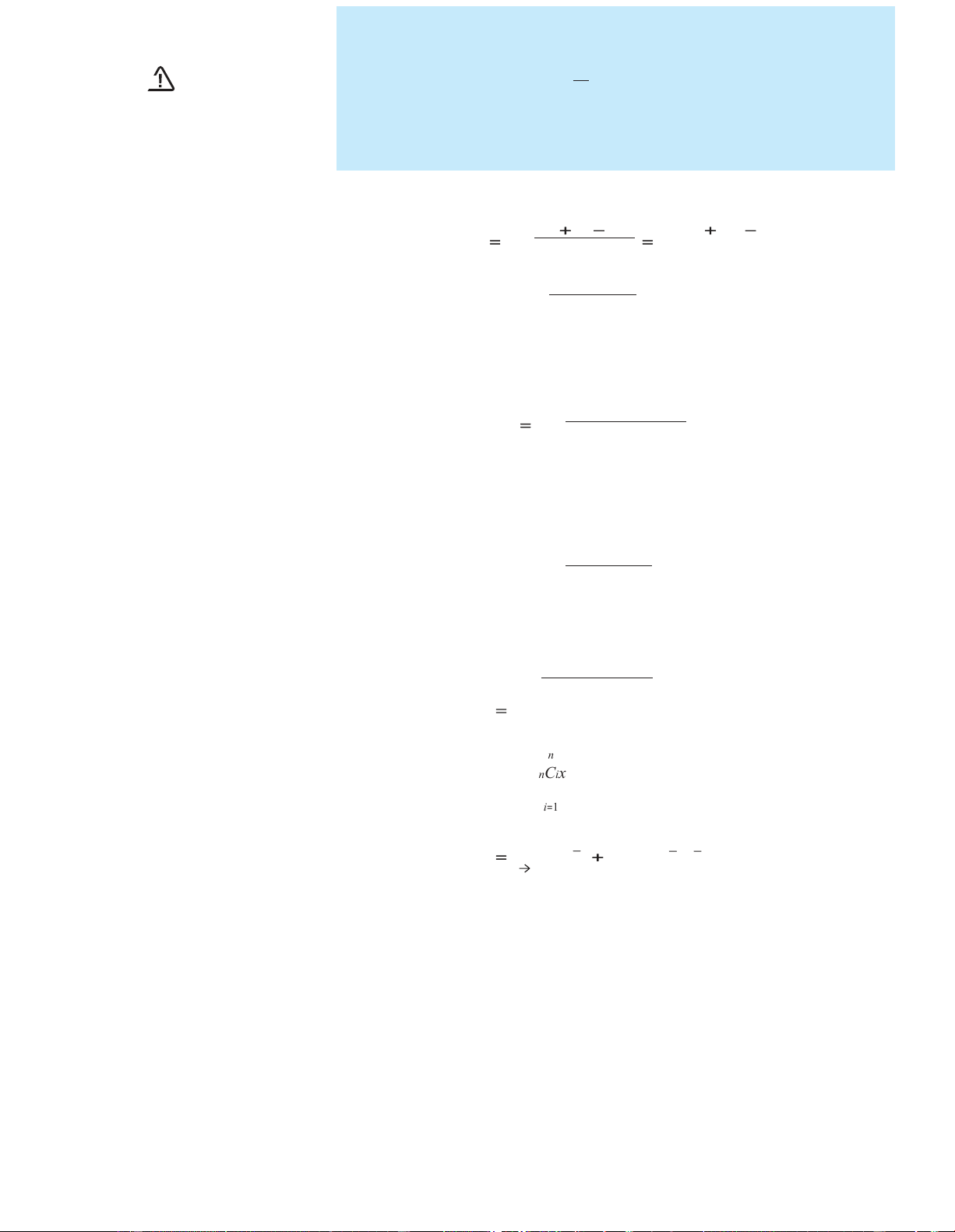
For the first of these we recall the binomial theorem of Section 9.2: n
(x + h)n = nCixn−ihi i=0
where the nCi are the binomial coefficients, whose precise descriptions, except for nC0
= 1 and nC1 = n, are not necessary here (but are given in Section 8.2). For the second we have n 1 x )
x i z n 1 i (z i 0 = zn − xn
which is easily verified by carrying out the multiplication using the rules for
manipulating summations given in Section 1.5. In fact, we have n 1 n 1 n 1
x i z n 1 i z
x i z n 1 i x i 0 i 0 i 0 (z − x) n 1 xizn−1−i n 1
x i z n i
xi+1zn−1−i i=0 i=0 n 1 n 2 z n
x i z n i
x i 1 z n 1 i x n i 1 i 0 = zn − xn
where the reader should check that the two summations in the second to last line really do cancel as shown. lOMoAR cPSD| 49519085
BASIC RULE 1 Derivative of xa If a is any real number, then
Section 11.2 Rules for Differentiation CAUTION a = a−1
There is a lot more to calculus than this rule. (x ) ax dx
That is, the derivative of a constant power of x is the exponent times x raised to a
power one less than the given power.
For n a positive integer, if f (x) = xn, the definition of the derivative gives f x ( x ) lim lim h 0 h h h ( h) f (x) (x h)n xn f
By our previous discussion on expanding ( 0
→x + h)n,→ n ( x ) lim h 0
nCixn−ihi − xn f i=0 →h n nCixn−ihi (1)= lim i=1 h→0h n
h nCixn−ihi−1 i=1 (2) lim h 0 → h (3) n
lim =nCixn−ihi−1 h 0 → i=1 n n 1 i lim nx h i 1 (4) n h 0 nCix i=2 (5)= nxn−1
where we justify the further steps as follows:
(1) The i = 0 term in the summation is nC0xnh0 = xn so it cancels with the separate, last, term: −xn.
(2) We are able to extract a common factor of h from each term in the sum.
(3) This is the crucial step. The expressions separated by the equal sign are limits as
h → 0 of functions of h that are equal for h = 0. 513 lOMoAR cPSD| 49519085 514 Chapter 11 Differentiation
(4) The i = 1 term in the summation is 1 1
nC1xn− h0 = nxn− . It is the only one that does not
contain a factor of h, and we separated it from the other terms.
(5) Finally, in determining the limit we made use of the fact that the isolated term is
independent of h; while all the others contain h as a factor and so have limit 0 as h → 0.
Now, using the z → x limit for the definition of the derivative and f (x) = xn, we have =
f (z) − f (x) =
zn −− xn f (x) lim
lim z→x z − x h→0 z x
By our previous discussion on factoring zn − xn, we have n 1
x i z n 1 i (z − x) f ( i x 0 ) lim z x z x → − n 1 (1) xizn−1−i lim z x → i=0 n 1 (2) = xixn−1−i i=0 n 1 (3) = xn−1 i=0 (4)= nxn−1
where this time we justify the further steps as follows:
(1) Here the crucial step comes first. The expressions separated by the equal sign are
limits as z → x of functions of z that are equal for z = x.
(2) The limit is given by evaluation because the expression is a polynomial in the variable z.
(3) An obvious rule for exponents is used.
(4) Each term in the sum is xn 1
− , independent of i, and there are n such terms. 506 50 3 EXAMPLE 2
Derivatives of Powers of x
a. By Basic Rule 1, d (x2) = 2x2−1 = 2x. dx
Tài liệu liên quan:
-
Kiem-toan - Bài tập kiểm toán căn bản có lời giải
65 33 -
Đề cương chi tiết học phần | môn toán cao cấp
734 367 -
Vi tích phân hàm một biến tính | Môn toán cao cấp
312 156 -
Bài giảng giáo trình giải tích | Môn toán cao cấp 2
319 160 -
Nội dung ôn tập chương 2 | Môn toán cao cấp
359 180