Chương 13: Linear Programming | Môn toán cao cấp

7/31/2020 lOMoAR cPSD| 47207194 Slide 8.1 Lecture 13 (19/5/2020) Chapter 8 Linear Programming
• Section 8.1. Graphical solution of linear programming problems (LPPs)
• Section 8.2. Applications of linear programming
Jacques, Mathematics for Economics and Business, 7th edition ' Pearson Education Limited 2012 Slide 8.2 Section 8.1. Graphical solution of linear programming problems (LPPs)
Identify the region defined by a linear inequality
Sketch the feasible region defined by simultaneous linear inequalities
Jacques, Mathematics for Economics and Business , 7 th edition ' Pearson Education Limited 2012 1 7/31/2020 lOMoAR cPSD| 47207194
Solve LPPs graphically
Special cases: many solutions and no finite solution Slide 8.3
Identify the region defined by a linear inequality
The graph of linear equation: dx
+ ey = f (1) is a straight line (d),
including al combinations (x, y) satisfying (1)
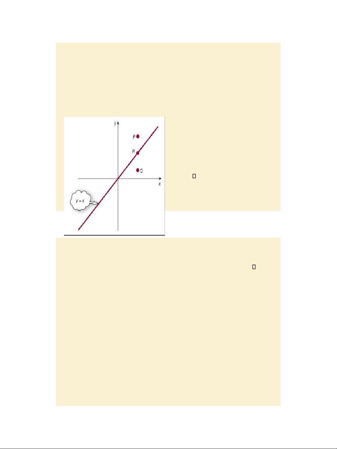
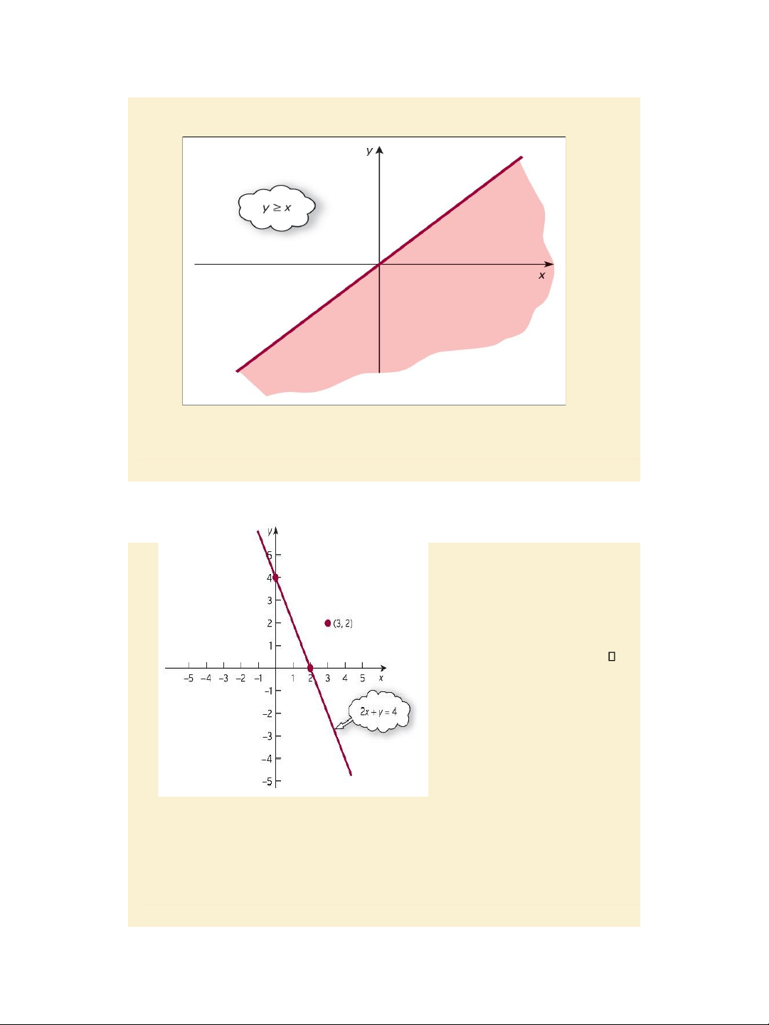
The region defined by inequality: dx + ey f (2) is a half plane
above or bel ow the straight line
(d). To test which one of these two
half planes satisfies (2) we pick a test point, say point P, not
belonging to (d). If point P satisfies
(2) then the half plane containing P
satisfies (2), otherwise the other half plane satisfies (2).
Similarly, we can identify the region Figure 8.1
defined by inequality dx + ey f (3).
Jacques, Mathematics for Economics and Business, 7th edition ' Pearson Education Limited 2012 Slide 8.4
Jacques, Mathematics for Economics and Business , 7 th edition ' Pearson Education Limited 2012 2 7/31/2020 lOMoAR cPSD| 47207194 Figure 8.2
The region defined by an inequality may be indicated pictorially by shading
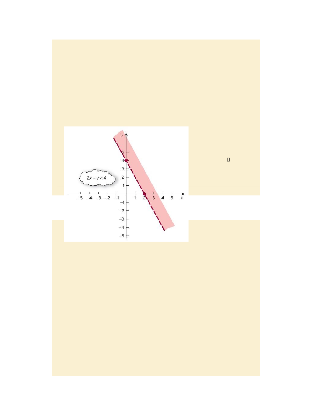
one half of the coordinate plane. Slide 8.5 Example, page 588: Sketch the region 2x + y < 4.
Step 1: Sketch the line 2x + y = 4.
Step 2: Pick a test point (3, 2)
and substitute x = 3 and y = 2
into the expression 2x + y = 2 3 + 2 = 8.
The test point does not satisfy the given inequality.
Step 3: The other half plane not
containing point (3, 2) satisfies the given inequality.
Jacques, Mathematics for Economics and Business , 7 th edition ' Pearson Education Limited 2012 3 7/31/2020 lOMoAR cPSD| 47207194
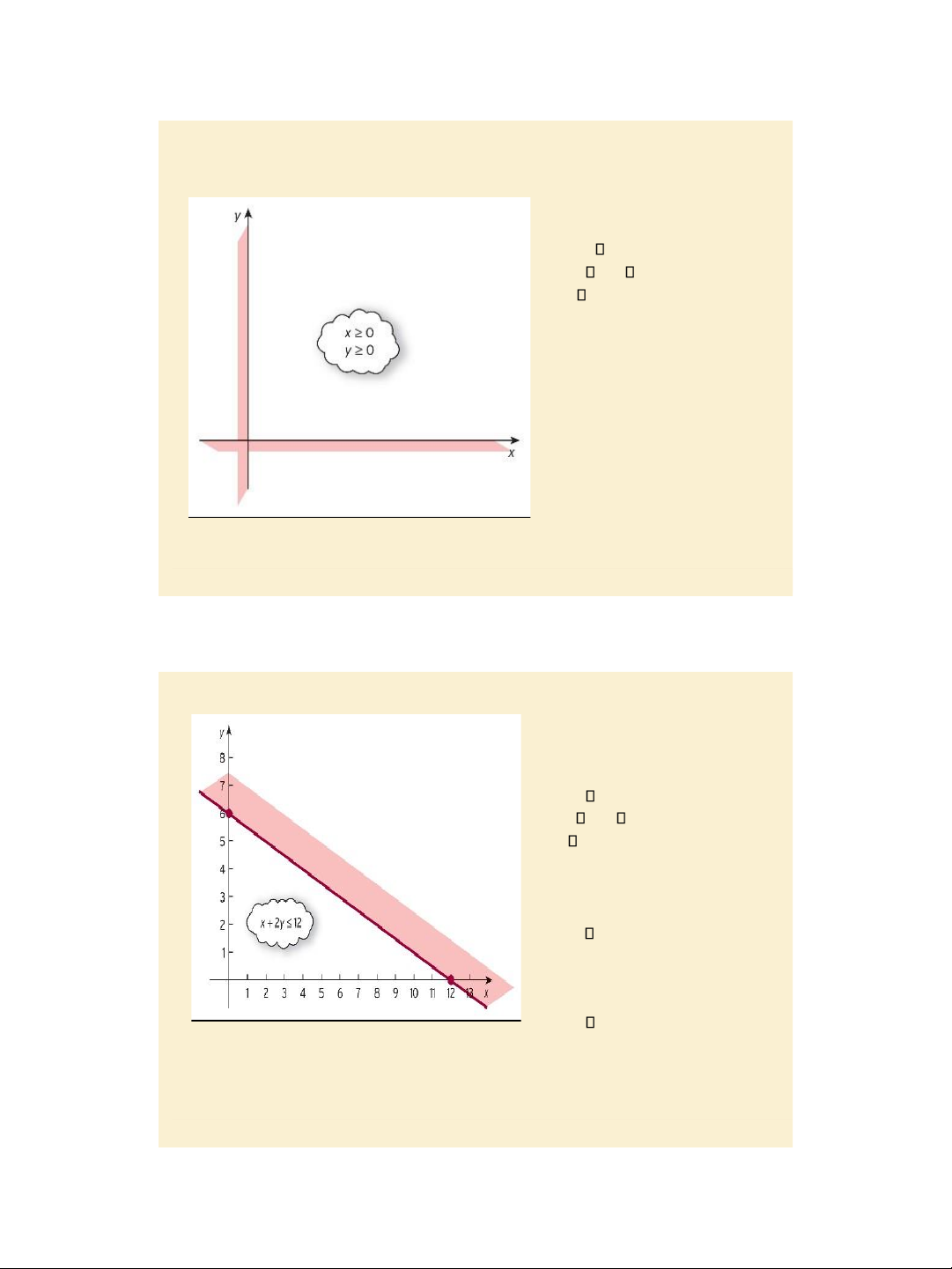
So, the region of interest lies Figure 8.3 bellow the straight line.
Jacques, Mathematics for Economics and Business, 7th edition ' Pearson Education Limited 2012 Slide 8.6 The region defined by inequality 2x + y < 4 Since the inequality is < (rather than ), al the points which lie on the straight line 2x + y = 4 do not belong to the region of interest and are not included in this region. To indicate this fact, we use a broken line for the boundary. Figure 8.4 Slide 8.7
Jacques, Mathematics for Economics and Business , 7 th edition ' Pearson Education Limited 2012 4 7/31/2020 lOMoAR cPSD| 47207194
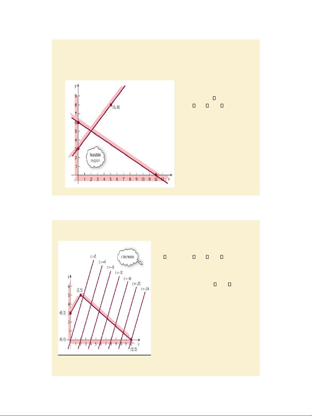
Sketch the feasible region defined by simultaneous linear inequalities Example, page 520 Sketch the feasible region: x + 2y 12 - x + y 3 x 0, y 0. Step 1: The last two inequalities mean that x and y are non-negative and hence we consider only points in the top righthand
quadrant (the first quadrant). Figure 8.5
Jacques, Mathematics for Economics and Business, 7th edition '
Pearson Education Limited 2012 Slide 8.8 Example, page 590 (continued) Sketch the feasible region: x + 2y 12 - x + y 3 x 0, y 0.
Step 2: In the first quadrant, sketch the region defined by: x + 2y 12.
Step 3: In the first quadrant, sketch the region defined by: - x + y 3.
Jacques, Mathematics for Economics and Business , 7 th edition ' Pearson Education Limited 2012 5 7/31/2020 lOMoAR cPSD| 47207194 Figure 8.6 Slide 8.9
Example, page 590 (contd.) Sketch the feasible region: x + 2y 12 - x + y 3 x 0, y 0. Step 4: Sketch the feasible region of interest (including
all points (x, y) satisfying the above four inequalities) that is the intersection of the regions found in steps 1, 2 and 3. Figure 8.7,
Jacques, Mathematics for Economics and Business, 7th edition ' Pearson Education Limited 2012 Slide 8.10
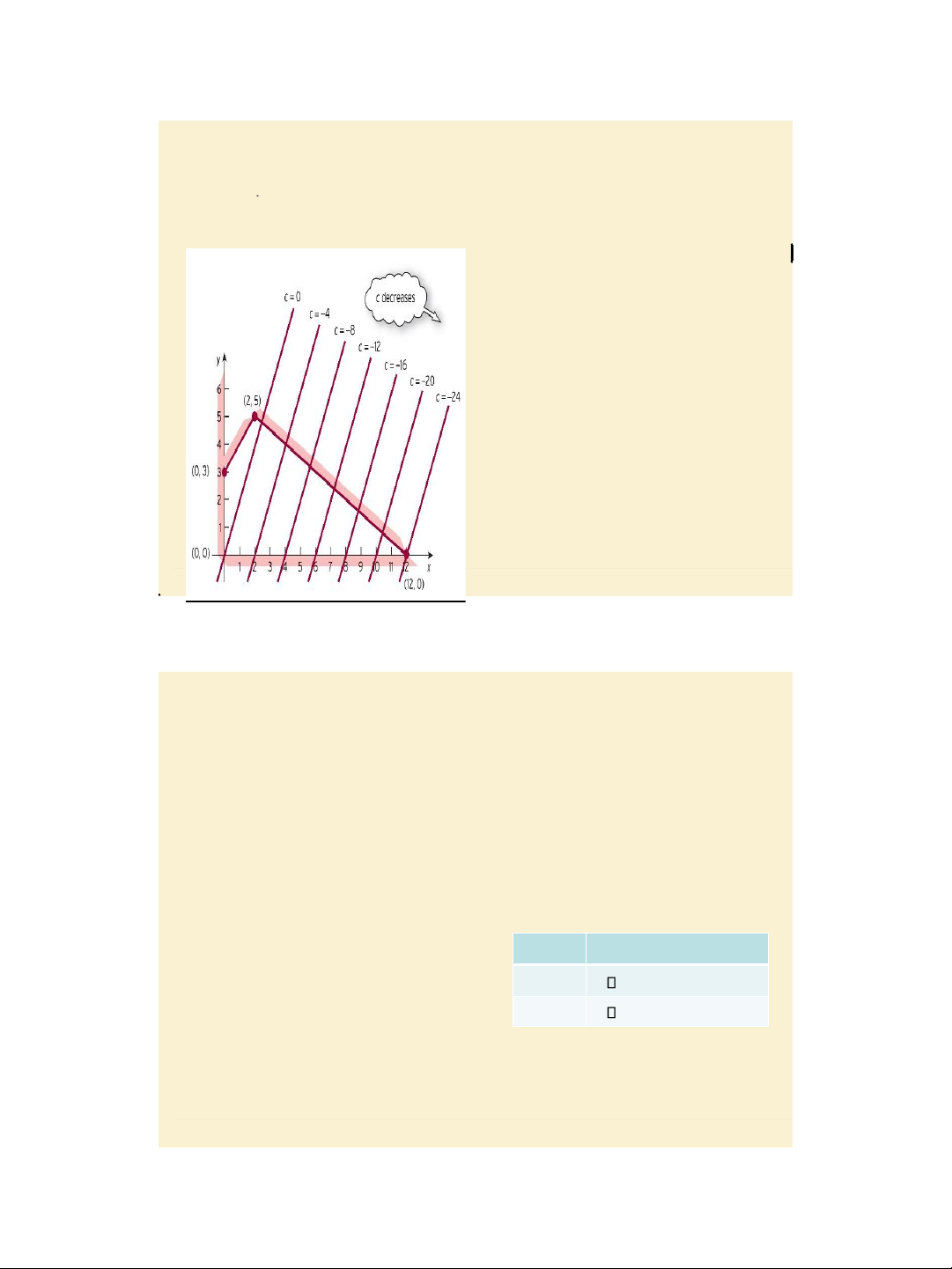
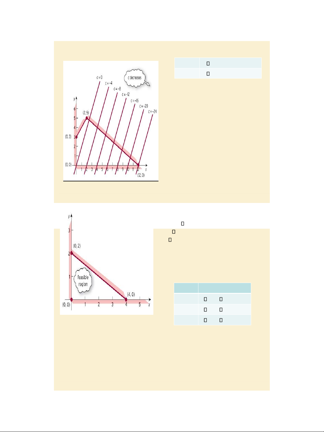
Solve LPPs graphically Example, page 592:
Solve the LPP: Minimize – 2x +
y subject to the constraints: x + 2y 12, - x + y 3 x 0, y 0.
Note: Here we have an objective function
to be minimized s.t. four constraints from
which 02 last ones are x 0, y 0 and
called non-negativity constraints. Isoquant line method to solve a LPP
Step 1: Sketch the feasible region defined by the 04 constraints
Step 2: Sketch line -2x + y = c for
different values of c (say c = 0, - 4, -8, …,
-24, …). They are parallel to each other,
and as c decreases from 0 to -24 the lines
sweep across the feasible region from left to right.
Jacques, Mathematics for Economics and Business , 7 th edition ' Pearson Education Limited 2012 6 7/31/2020 lOMoAR cPSD| 47207194 Figure 8.8
Step 3: The minimum value of the o.f. is Slide 8.11
value -24, achieved at (x, y) = (12, 0).
Solve LPPs graphically
Example, page 592: Solution (contd.)
Step 3: The minimum value of c, so that
the line – 2x + y = c still touches
(intersects) the feasible region, is c =
24. The solution to the LPP is Min (-2x +
y) = -24 achieved at (x, y) = (12, 0).
Note: The optimal value of the objective
function is attained at one of the corners
of the feasible region (in case the feasible region is bounded).
Corner point method to solve a LPP:
Step 1: Sketch the feasible region D.
Step 2: Identify al the corners of D and their coordinates.
Step 3: Evaluate the objective function at
the corners and choose the one which
has the maximum or minimum value. Figure 8.8
Jacques, Mathematics for Economics and Business, 7th edition ' Pearson Education Limited 2012 Slide 8.12
Solve LPPs graphically
Corner Objective function A(0, 0) -2 0 + 0 = 0 B(0, 3) -2 0 + 3 = 3
Jacques, Mathematics for Economics and Business , 7 th edition ' Pearson Education Limited 2012 7 7/31/2020 lOMoAR cPSD| 47207194 C(2, 5) -2 2 + 5 = 1 D(12, 0) -2 12+ 0 = -24
Example, pages 592-595: Solution
Step 1: Sketch the feasible region D.
Step 2: Identify al the corners of D and
their coordinates: A(0, 0), B(0, 3), C(2, 5) and D (12, 0).
Step 3: Evaluate the objective function at the corners
We choose point D(12, 0), that is (x, y) =
(12, 0) at which o.f. is minimized and the minimum value is -24.
Figure 8.8 If we want to maximize the o.f. then we choose point B(0, 3). Slide 8.13
Solve LPPs graphically Example, pages 595 - 596:
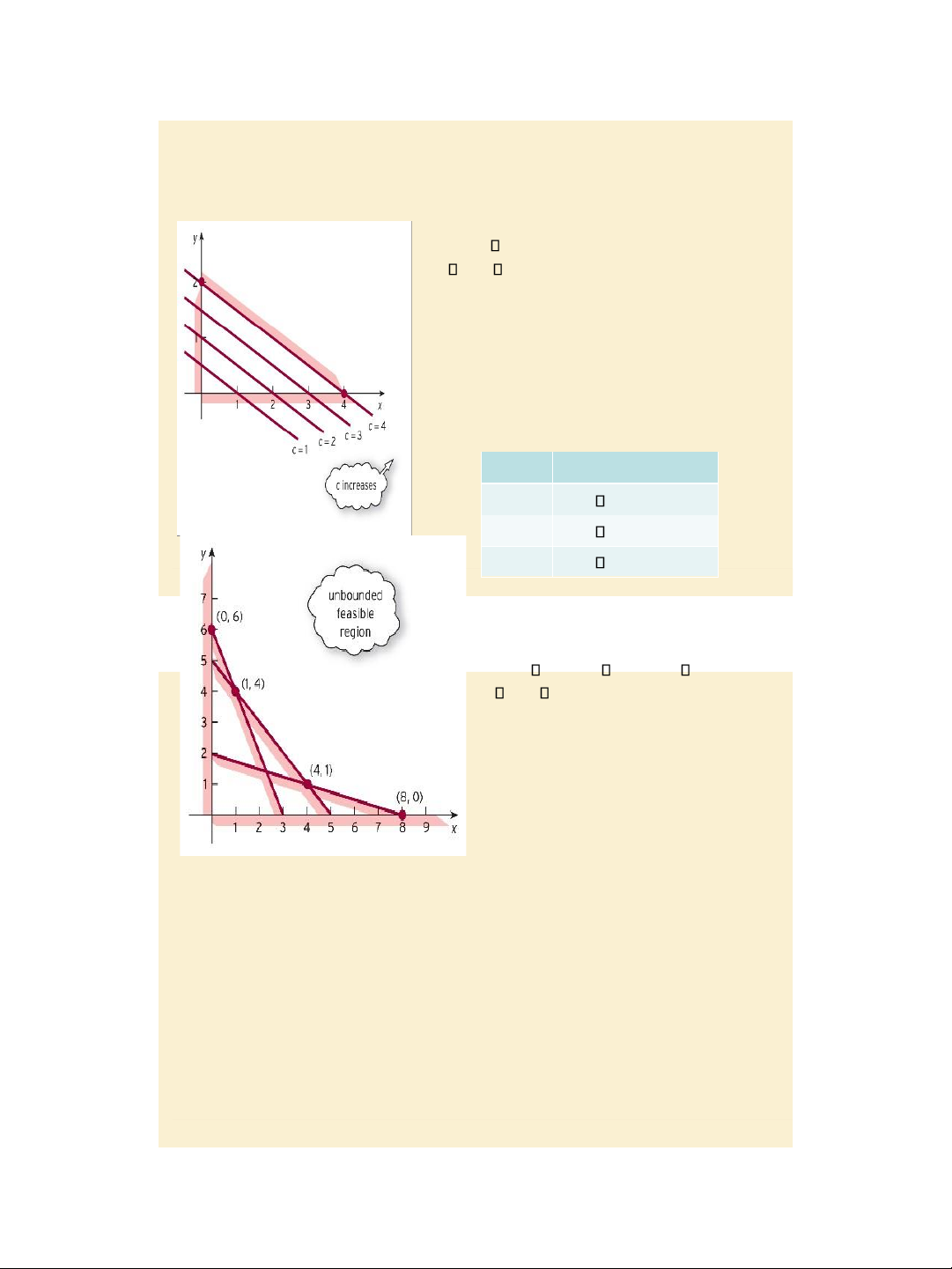
Maximize 5x + 3y subject to the constraints: 2x + 4y 8, x 0, y 0.
Step 1: Sketch the feasible region D. Step
2: Identify all the corners of D and their
coordinates: A(0, 0), B(0, 2) and C(4, 0).
Step 3: Evaluate the objective function at the
Corner Objective function A(0, 0) 5 0 + 3 0 = 0 B(0, 2) 5 0 + 3 2 = 6 corners A, B and C C(4, 0) 5 4 + 3 0 = 20 At (x, y) =
(4, 0) the o.f. is maximized and Figure 8.9 the maximum value is 20.
Jacques, Mathematics for Economics and Business, 7th edition ' Pearson Education Limited 2012
Jacques, Mathematics for Economics and Business , 7 th edition ' Pearson Education Limited 2012 8 7/31/2020 lOMoAR cPSD| 47207194 Slide 8.14
Solve LPPs graphically: many solutions Example, pages 597 - 598:
Maximize x + 2y subject to the constraints: 2x + 4y 8, x 0, y 0.
Step 1: Sketch the feasible region D.
Step 2: Identify al the corners of D and their
coordinates: A(0, 0), B(0, 2) and C(4, 0).
Step 3: Evaluate the objective function at the corners A, B and C
At (x, y) = (4, 0) and (x, y) = (0, 2) the o.f. is
Figure 8.10maximized and the maximum value is 4. Slide 8.15
Corner Objective function Solve LPPs A(0, 0) 0 + 2 0 = 0 B(0, 2) 0 + 2 2 = 4 C(4, 0) 4 + 2 0 = 4
graphically: unbounded feasible region and no finite solution
Example, pages 598 - 599: Maximize
3x + 2y subject to the constraints: x + 4y 8, x + y 5, 2x + y 6, x 0, y 0.
Step 1: Sketch the feasible region D.
Step 2: Identify al the corners of D and
their coordinates: A(0, 6), B(1, 4), C(4, 1) and D(8, 0).
Step 3: The objective function at the corners A, B, C and D has
correspondingly values: 12, 11, 14 and 24.
Since the feasible region is unbounded,
Jacques, Mathematics for Economics and Business , 7 th edition ' Pearson Education Limited 2012 9 7/31/2020 lOMoAR cPSD| 47207194
the comparison of values of the o.f. at Figure 8.11
different corners has no sense, i.e. the
corner method can not be of use.
Jacques, Mathematics for Economics and Business, 7th edition ' Pearson Education Limited 2012 Slide 8.16
Solve LPPs graphically:
unbounded feasible region and no
finite solution Example, pages 598 -
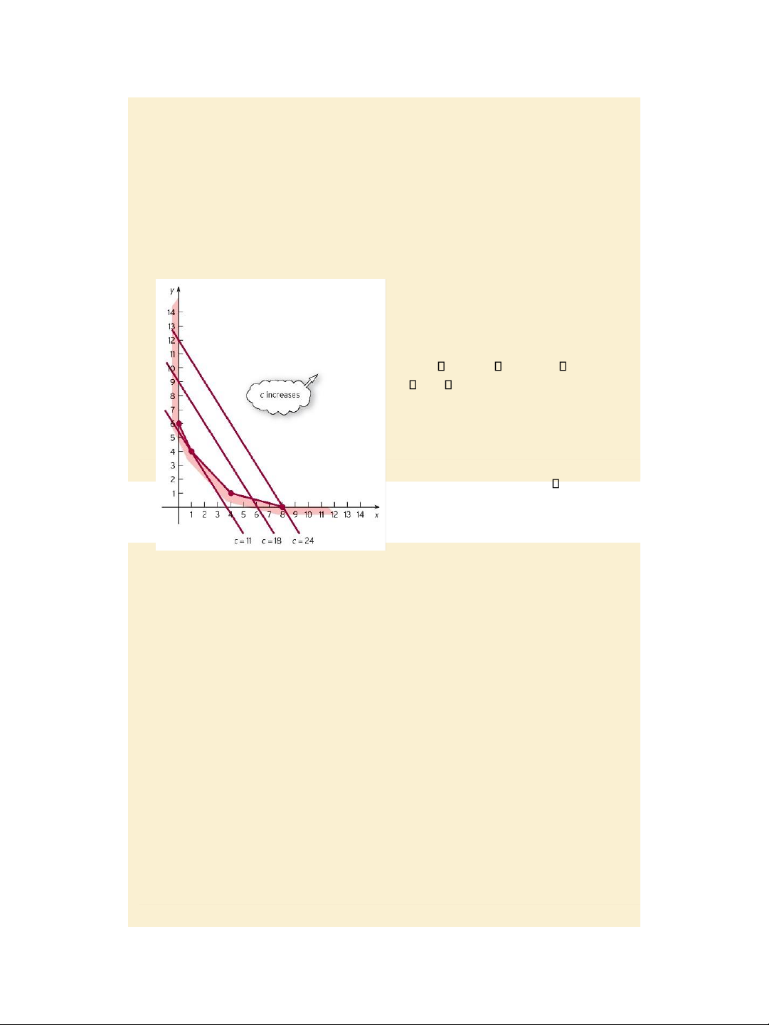
599 (contd.): Maximize 3x + 2y subject to the constraints: x + 4y 8, x + y 5, 2x + y 6, x 0, y 0.
Isoquant line method to solve the LPP
Step 1: Sketch the feasible region D.
Step 2: Sketch line 3x + 2y = c for
different values of c (say c = 0, 5, 11,
…). They are parallel to each other, and
as c increases from 11 to + , the lines
sweep across the feasible region from left to right.
Step 3: The objective function has no finite solution. Figure 8.12, page 530
Key terms: page 600, Exercise 8.1*: problems 5, 6, 7 page 602. Slide 8.17 Section 8.2.
Applications of linear programming
Identify the unknowns in a LPP
Find an expression for the objective function and
decide whether it should be minimized or maximized
Write down all the constraints
Solve LPPs expressed in words and check that the
Jacques, Mathematics for Economics and Business , 7 th edition ' Pearson Education Limited 2012 10 7/31/2020 lOMoAR cPSD| 47207194 answer makes sense
Jacques, Mathematics for Economics and Business, 7th edition ' Pearson Education Limited 2012 Slide 8.18 Example:
A manufacturer produces 02 kinds of good, A and B, for which
demand exceeds capacity. The production costs for A and B are
$6 and $3, respectively, and the corresponding selling prices
are $7 and $4. The transport costs for each good of type A and
B are 20 cents and 30 cents, respectively. Due to a bank loan
limit, weekly production costs and weekly transport costs can
not exceed $2700 and $120, respectively.
How should the manufacturer arrange production to maximize profit?
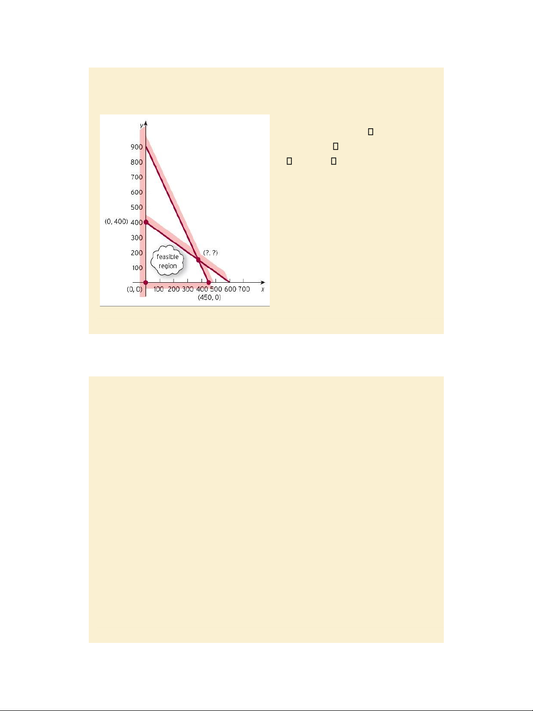
Identifying unknowns: x = number of goods of type A / week,
y = number of goods of type B/ week. Stating the LPP: Maximize 0.8x + 0.7y s.t. 6x + 3y 2700 0.2x + 0.3y 120 x 0 and y 0. Slide 8.19
Jacques, Mathematics for Economics and Business , 7 th edition ' Pearson Education Limited 2012 11 7/31/2020 lOMoAR cPSD| 47207194 Example (contd.) Maximize 0.8x + 0.7y s.t. 6x + 3y 2700 0.2x + 0.3y 120 x 0 and y 0. Solution
Step 1: Sketch the feasible region.
Step 2: Identify the corner points of the
region: A (0, 0), B (0, 400), C(375, 150), D(450, 0).
Step 3: Evaluate the objective function
values at corners A, B, C and D to get
0, 280, 405 and 360 correspondingly.
So the maximum weekly profit is $405,
which occurs when 375 goods of type A and 150 goods of type B are manufactured.
Jacques, Mathematics for Economics and Business, 7th edition ' Pearson Education Limited 2012 Slide 8.20 Example, pages 604-606
A craft studio makes glass bowls and plates, and it can sell all of the products
that it makes each week. Glassware is made in two stages. In the first stage
molten glass is taken from a furnace and placed at the end of a blowpipe.
Skil ed glassblowers then mould the glass into the desired shape. During the
second stage the glass is allowed to cool in a controlled way inside a second
furnace (called an annealer) which helps to reduce stress and prevent the
glass from cracking. The studio employs two glassblowers who each work a
35-hour week, and the total time available each week for annealing is 130
hours. The main raw material used in glassmaking is silica sand, and the
studio orders 45 kg each week. A glass bowl and plate each require 1 kg of
sand. It takes a glassblower two hours to make a bowl and one hour to make a
plate. The time needed to cool a bowl in an annealer is four hours and a plate
requires one hour. The profit made from selling a bowl and a plate is $150 and
$100, respectively. How should the manufacturer arrange production to maximize profit?
Identifying unknowns: x = number of bowls, y = number of plates.
Jacques, Mathematics for Economics and Business , 7 th edition ' Pearson Education Limited 2012 12 7/31/2020 lOMoAR cPSD| 47207194
Stating the LPP: Maximize 150x + 100y (profit)
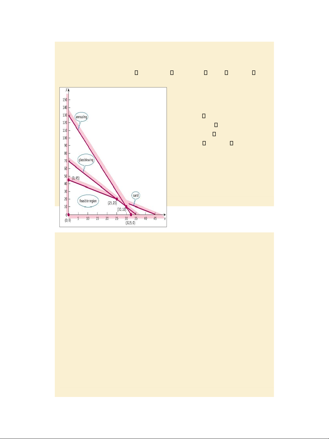
s.t.: 2x + y 70; 4x + y 130; x + y 45; x 0 and y 0. Slide 8.21 Example (contd.)
Maximize 150x + 100y (profit) s.t.: 2x + y 70 (glassblowing time) 4x + y 130 (annealing
time) x + y 45 (mass of silica sand) x 0 and y 0. Solution
Step 1: Sketch the feasible region.
Step 2: Identify the corner points of the
region: A (0, 0), B (0, 45), C(25, 20), D(30, 10) and E (32.5, 0).
Step 3: Evaluate the objective function
values at corners A, B, C , D and E to
get 0, 4500, 5750, 5500, 4875, respectivey.
So the maximum weekly profit is
$5750, which occurs when x = 25
(bowls) and y = 20 (plates) are Figure 8.13 manufactured.
Jacques, Mathematics for Economics and Business, 7th edition ' Pearson Education Limited 2012 Slide 8.22
Jacques, Mathematics for Economics and Business , 7 th edition ' Pearson Education Limited 2012 13 7/31/2020 lOMoAR cPSD| 47207194 Example, pages 608 - 611
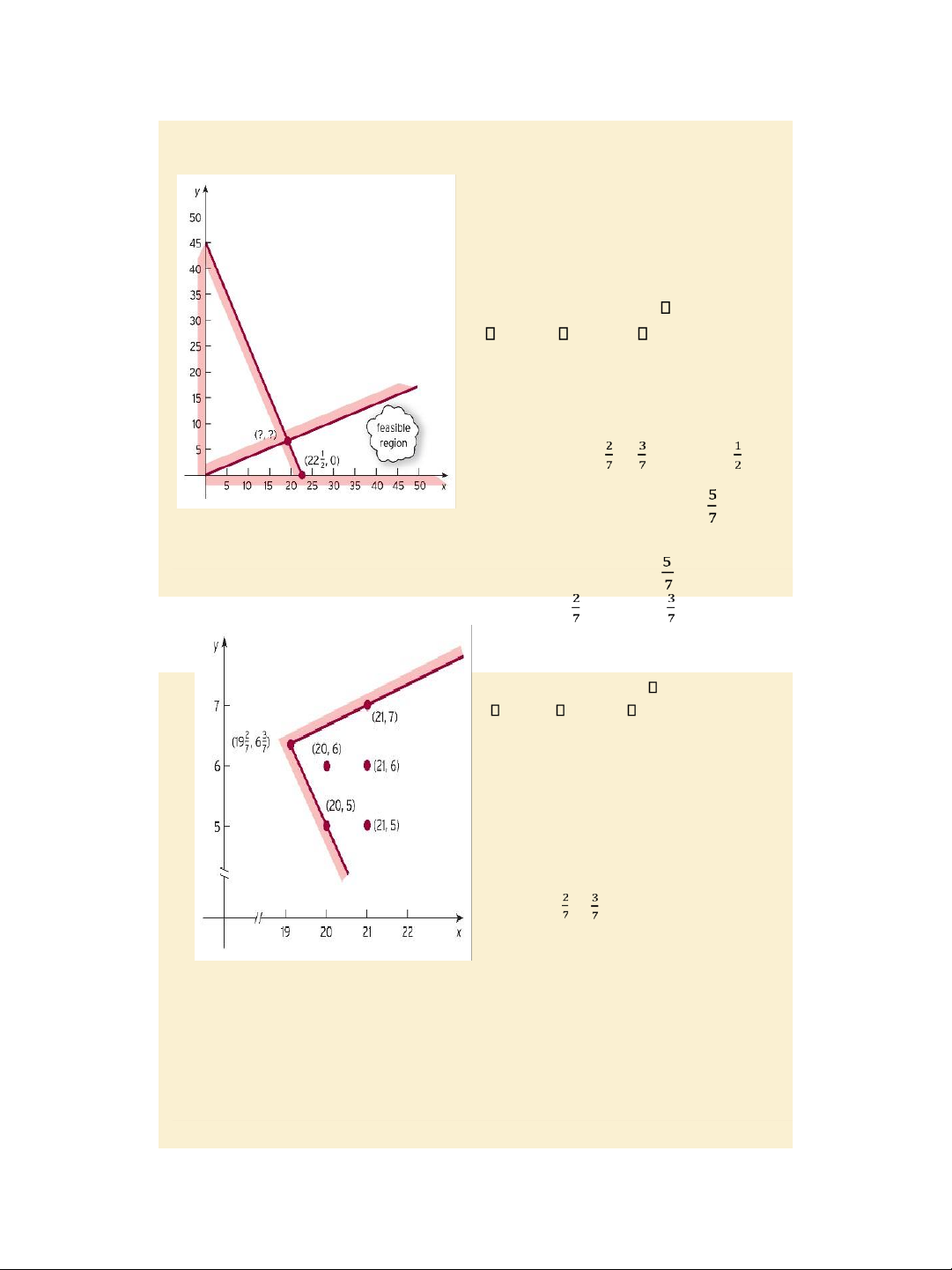
Identifying unknowns: x = ful -time staff, y = part-time staff. Stating LPP: Minimize 800x + 320y s.t. 40x + 20y 900 y x/3, x 0 and y 0. Solution (using the corner point method)
Step 1: Sketch the feasible region.
Step 2: Identify the corner points of
the region: A (19 , 6 ) and B(22 , 0) Step 3: Evaluate the objective function values at A and B to get 17485 and Figure 8.14
Note: To be more exact, the 18000. The minimum cost is $17485 isoquant line
method should be used when x = 19 and y = 6 . Slide 8.23 Example, pages 608 - 611 (contd.) LPP: Minimize 800x + 320y s.t. 40x + 20y 900 y x/3, x 0 and y 0.
Moreover, x and y should be integers (whole numbers)
Solution (using the corner point method)
Step 1: Sketch the feasible region.
Step 2: Identify some feasible points with
integer coordinates of the region which
are close / neighbor to the corner optimal
point A (19 , 6 ) : they are (20, 5), (20,
6), (21, 5), (21, 6), (21, 7) ..
Step 3: Evaluate the objective function Figure 8.15
values at the above points to find the
Key terms: page 612, Exercise
minimum is $17600 when x = 20 and
8.2*: problems 4, 5, pages 614 - 615 y = 5.
Formal mathematics: page 617
Jacques, Mathematics for Economics and Business, 7th edition ' Pearson Education Limited 2012
Jacques, Mathematics for Economics and Business , 7 th edition ' Pearson Education Limited 2012 14 7/31/2020 lOMoAR cPSD| 47207194 Slide 8.24
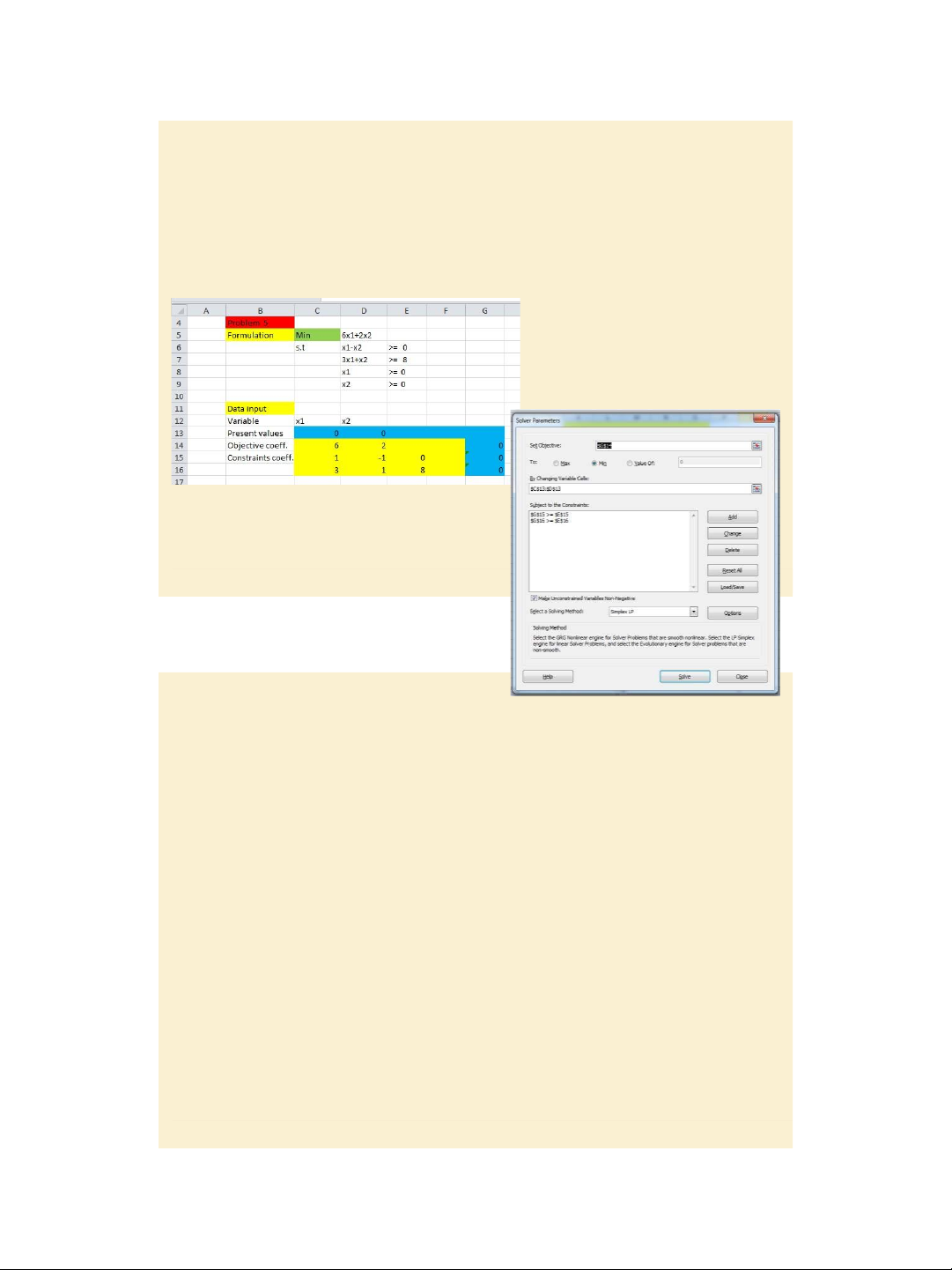
Using Excel Solver to solve a LPP Exercise 8.1* Problem 5, page 602
Jacques, Mathematics for Economics and Business , 7 th edition ' Pearson Education Limited 2012 15