Econ Final: Regression Analysis and Time-Series Modelling Notes | Môn Econometrics with Financial Application - Trường Đại học Quốc tế, Đại học Quốc gia Thành phố Hồ Chí Minh

lOMoAR cPSD| 58583460
Chap 4: Further Development and Analysis of the Classical Linear Regression Model
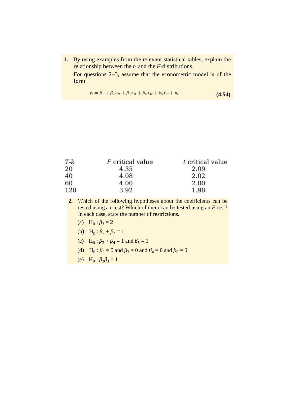
It can be proved that a t-distribution is just a special case of the more general F-distribution.
The square of a t-distribution with T-k degrees of freedom will be identical to an F-distribution
with (1,T-k) degrees of freedom. But remember that if we use a 5% size of test, we will look
up a 5% value for the F-distribution because the test is 2-sided even though we only look in
one tail of the distribution. We look up a 2.5% value for the t distribution since the test is 2- tailed.
Examples at the 5% level from tables a.
We could use an F- or a t- test for this one since it is a single hypothesis involving only
one coefficient. We would probably in practice use a t-test since it is computationally simpler
and we only have to estimate one regression. There is one restriction. b.
Since this involves more than one coefficient, we should use an F-test. There is one restriction. c.
Since we are testing more than one hypothesis simultaneously, we would use an F-test. There are 2 restrictions. d.
As for (c), we are testing multiple hypotheses so we cannot use a t-test. We have 4 restrictions. e.
Although there is only one restriction, it is a multiplicative restriction. We therefore
cannot use a t-test or an F-test to test it. In fact we cannot test it at all using the methodology
that has been examined in this chapter. lOMoAR cPSD| 58583460
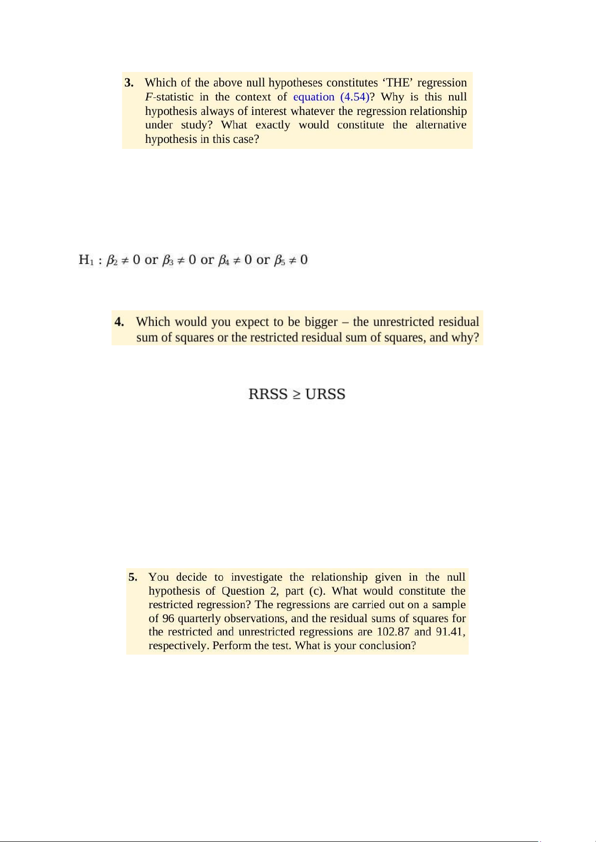
THE regression F-statistic would be given by the test statistic associated with hypothesis iv)
above. We are always interested in testing this hypothesis since it tests whether all of the
coefficients in the regression (except the constant) are jointly insignificant. If they are then we
have a completely useless regression, where none of the variables that we have said influence
y actually do. So we would need to go back to the drawing board! The alternative hypothesis is:
Note the form of the alternative hypothesis: “or” indicates that only one of the components of
the null hypothesis would have to be rejected for us to reject the null hypothesis as a whole.
The restricted residual sum of squares will always be at least as big as the unrestricted residual sum of squares i.e.
To see this, think about what we were doing when we determined what the regression
parameters should be: we chose the values that minimize the residual sum of squares. We said
that OLS would provide the “best” parameter values given the actual sample data. Now when
we impose some restrictions on the model, so that they cannot all be freely determined, then
the model should not fit as well as it did before. Hence the residual sum of squares must be
higher once we have imposed the restrictions; otherwise, the parameter values that OLS chose
originally without the restrictions could not be the best.
In the extreme case (very unlikely in practice), the two sets of residual sum of squares could be
identical if the restrictions were already present in the data, so that imposing them on the model
would yield no penalty in terms of loss of fit. lOMoAR cPSD| 58583460 lOMoAR cPSD| 58583460 lOMoAR cPSD| 58583460 lOMoAR cPSD| 58583460
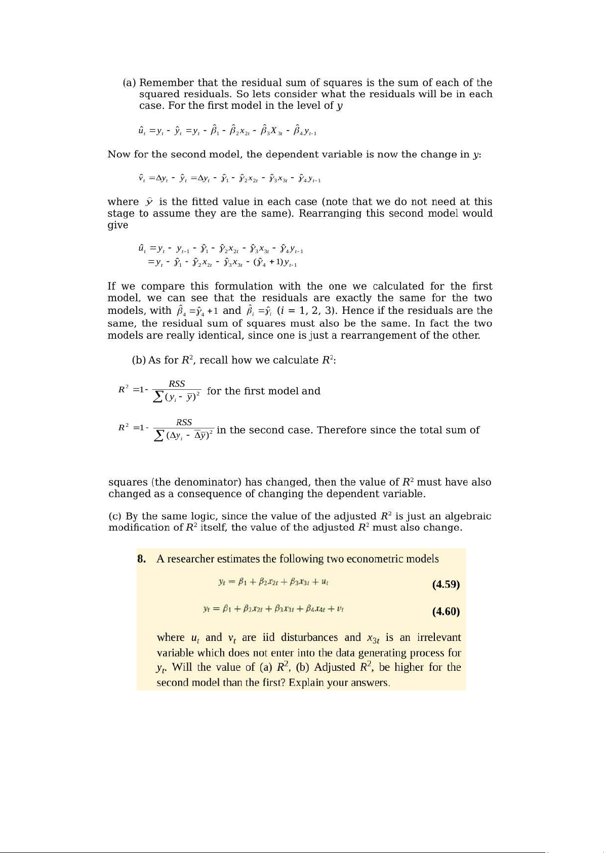
R-squared (R2) is a number that tells you how well the independent variable(s) in a statistical
model explain the variation in the dependent variable. It ranges from 0 to 1, where 1 indicates
a perfect fit of the model to the data. R-squared values range from 0 to 1 and are commonly
stated as percentages from 0% to 100%.
Quantile regression provides an alternative to ordinary least squares (OLS) regression and
related methods, which typically assume that associations between independent and dependent
variables are the same at all levels. Quantile methods allow the analyst to relax the common
regression slope assumption. In OLS regression, the goal is to minimize the distances between
the values predicted by the regression line and the observed values. In contrast, quantile
regression differentially weights the distances between the values predicted by the regression
line and the observed values, then tries to minimize the weighted distances.
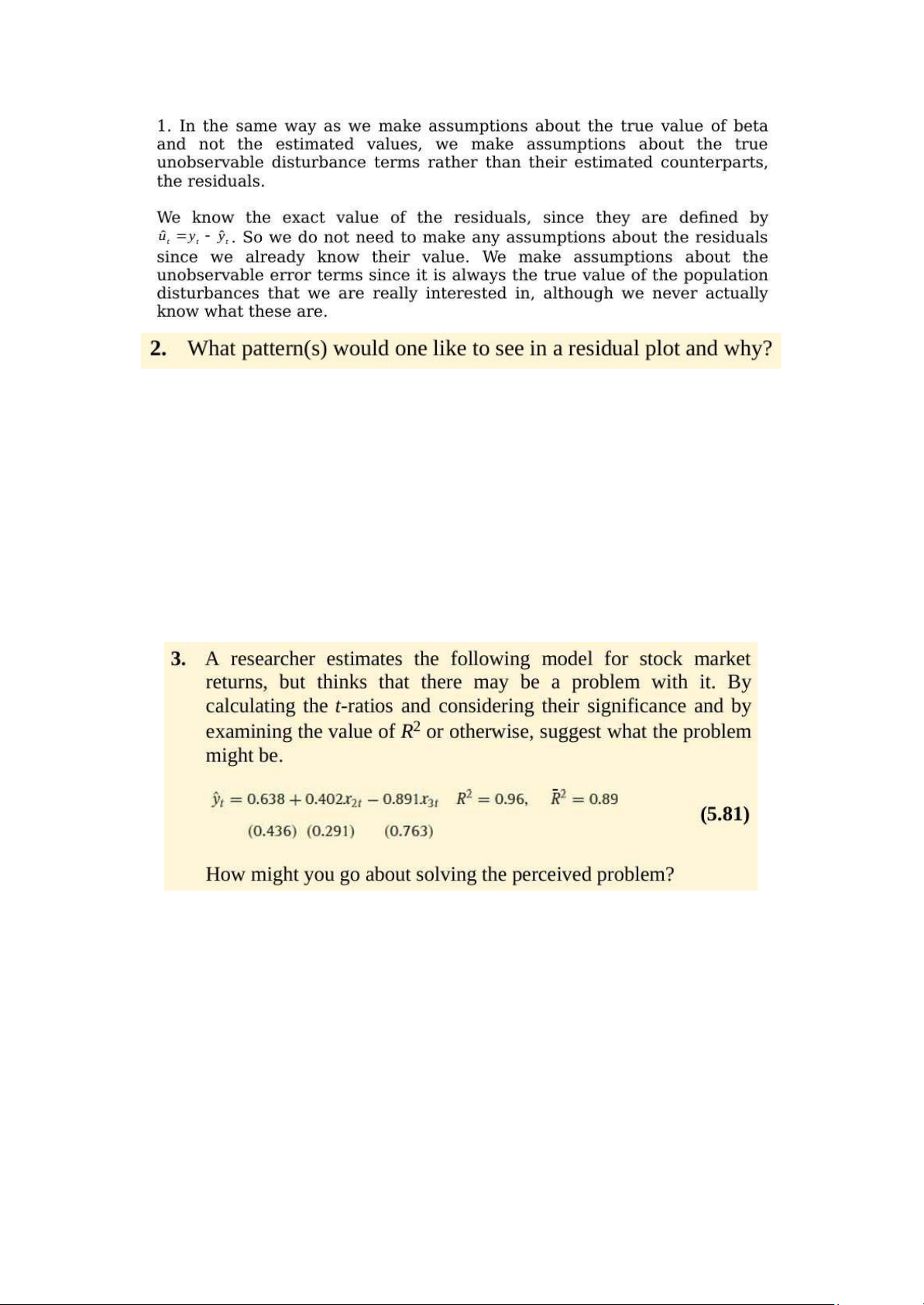
Chap 5: Classical Linear Regression Model Assumptions and Diagnostic Tests lOMoAR cPSD| 58583460
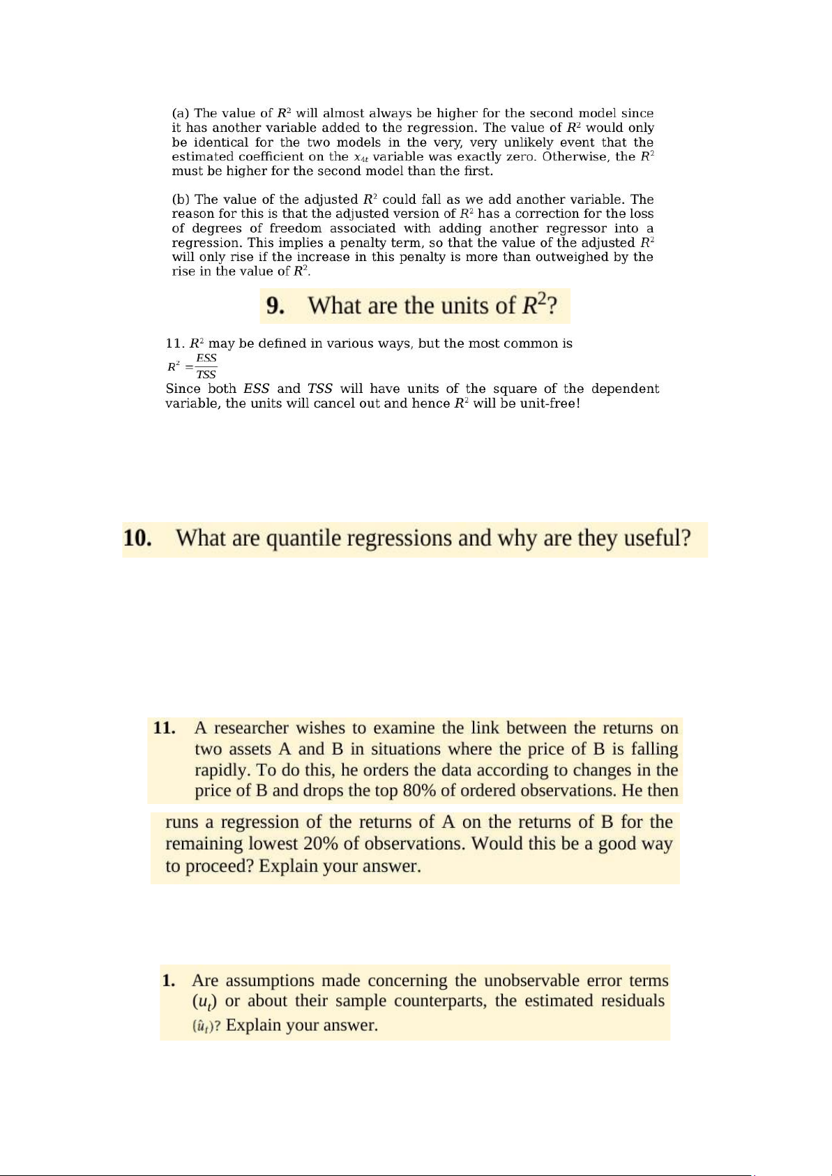
We would like to see no pattern in the residual plot! If there is a pattern in the residual plot, this
is an indication that there is still some “action” or variability left in yt that has not been
explained by our model. This indicates that potentially it may be possible to form a better
model, perhaps using additional or completely different explanatory variables, or by using lags
of either the dependent or of one or more of the explanatory variables. Recall that the two plots
shown on pages 157 and 159, where the residuals followed a cyclical pattern, and when they
followed an alternating pattern are used as indications that the residuals are positively and
negatively autocorrelated respectively.
Another problem if there is a “pattern” in the residuals is that, if it does indicate the presence
of autocorrelation, then this may suggest that our standard error estimates for the coefficients
could be wrong and hence any inferences we make about the coefficients could be misleading. lOMoAR cPSD| 58583460 lOMoAR cPSD| 58583460 the case ?
b. The coefficient estimates would still be the “correct” ones (assuming that the other
assumptions required to demonstrate OLS optimality are satisfied), but the problem would
be that the standard errors could be wrong. Hence if we were trying to test hypotheses about
the true parameter values, we could end up drawing the wrong conclusions. In fact, for all of
the variables except the constant, the standard errors would typically be too small, so that we
would end up rejecting the null hypothesis too many times.
c. There are a number of ways to proceed in practice, including -
Using heteroskedasticity robust standard errors which correct for the problem by
enlarging the standard errors relative to what they would have been for the situation where the
error variance is positively related to one of the explanatory variables. -
Transforming the data into logs, which has the effect of reducing the effect of large
errors relative to small ones. lOMoAR cPSD| 58583460 a.
This is where there is a relationship between the ith and jth residuals. Recall that one of
the assumptions of the CLRM was that such a relationship did not exist. We want our residuals
to be random, and if there is evidence of autocorrelation in the residuals, then it implies that
we could predict the sign of the next residual and get the right answer more than half the time on average! b.
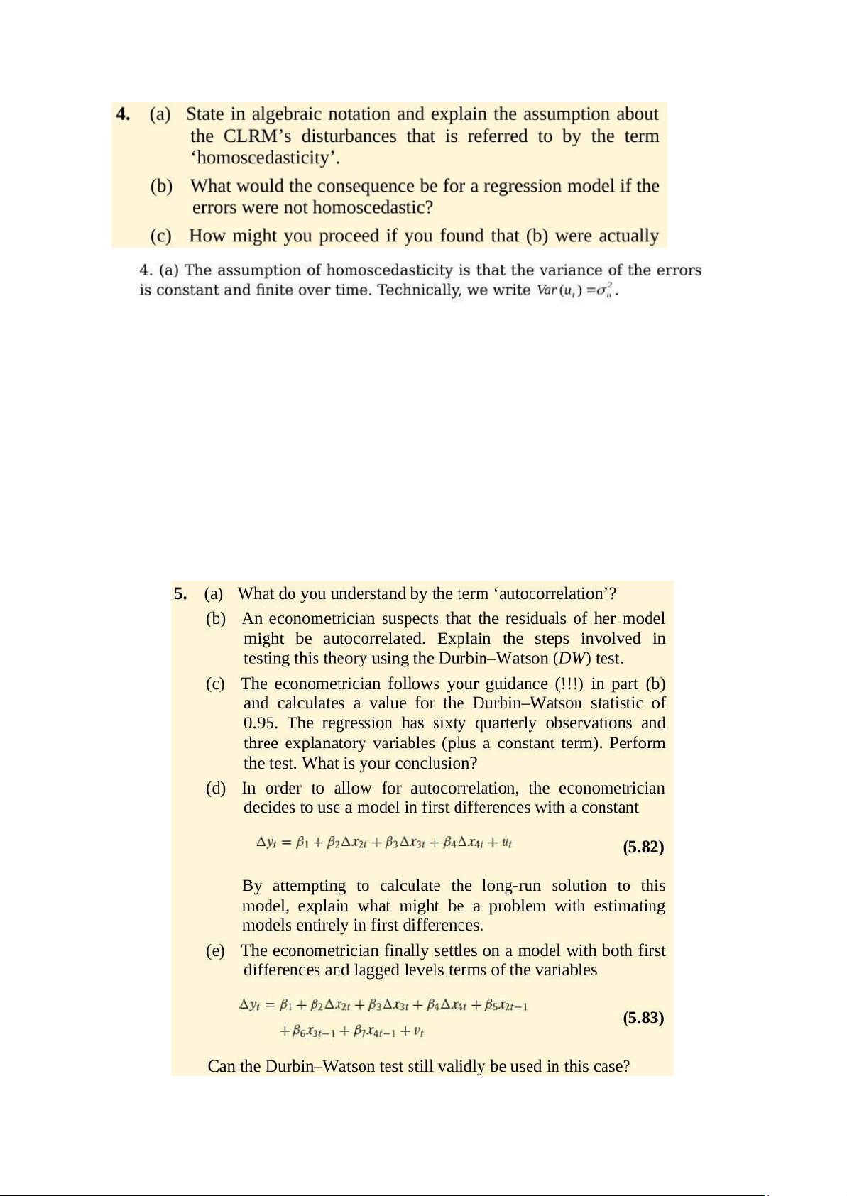
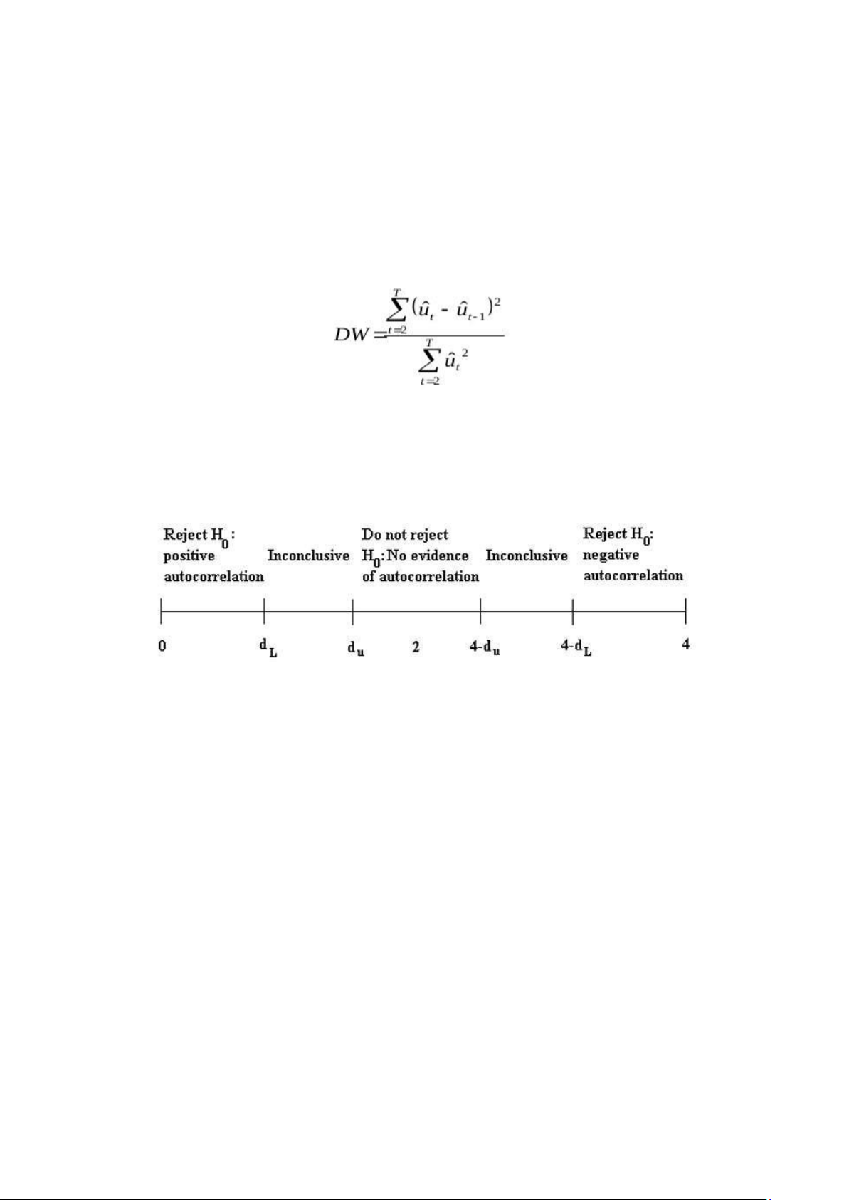
The Durbin Watson test is a test for first order autocorrelation. The test is calculated as
follows. You would run whatever regression you were interested in, and obtain the residuals. Then calculate the statistic
You would then need to look up the two critical values from the Durbin Watson tables, and
these would depend on how many variables and how many observations and how many
regressors (excluding the constant this time) you had in the model.
The rejection / non-rejection rule would be given by selecting the appropriate region from the following diagram: c.
We have 60 observations, and the number of regressors excluding the constant term is
3. The appropriate lower and upper limits are 1.48 and 1.69 respectively, so the Durbin Watson
is lower than the lower limit. It is thus clear that we reject the null hypothesis of no
autocorrelation. So it looks like the residuals are positively autocorrelated. d.
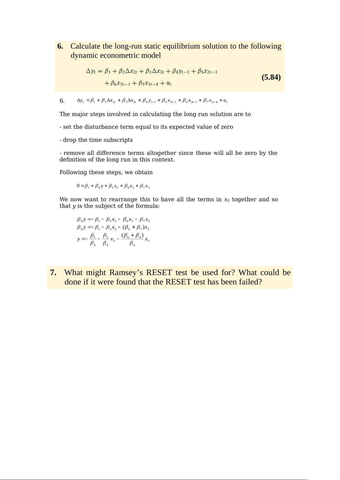
The problem with a model entirely in first differences, is that once we calculate the long
run solution, all the first difference terms drop out (as in the long run we assume that the values
of all variables have converged on their own long run values so that yt = yt-1 etc.) Thus when
we try to calculate the long run solution to this model, we cannot do it because there isn’t a
long run solution to this model! e.
The answer is yes, there is no reason why we cannot use Durbin Watson in this case.
You may have said no here because there are lagged values of the regressors (the x variables)
variables in the regression. In fact this would be wrong since there are no lags of the
DEPENDENT (y) variable and hence DW can still be used. lOMoAR cPSD| 58583460
The last equation above is the long run solution.
Ramsey’s RESET test is a test of whether the functional form of the regression is appropriate.
In other words, we test whether the relationship between the dependent variable and the
independent variables really should be linear or whether a non-linear form would be more
appropriate. The test works by adding powers of the fitted values from the regression into a
second regression. If the appropriate model was a linear one, then the powers of the fitted values
would not be significant in this second regression.
If we fail Ramsey’s RESET test, then the easiest “solution” is probably to transform all of the
variables into logarithms. This has the effect of turning a multiplicative model into an additive one.
If this still fails, then we really have to admit that the relationship between the dependent
variable and the independent variables was probably not linear after all so that we have to either
estimate a non-linear model for the data (which is beyond the scope of this course) or we have
to go back to the drawing board and run a different regression containing different variables. lOMoAR cPSD| 58583460 a.
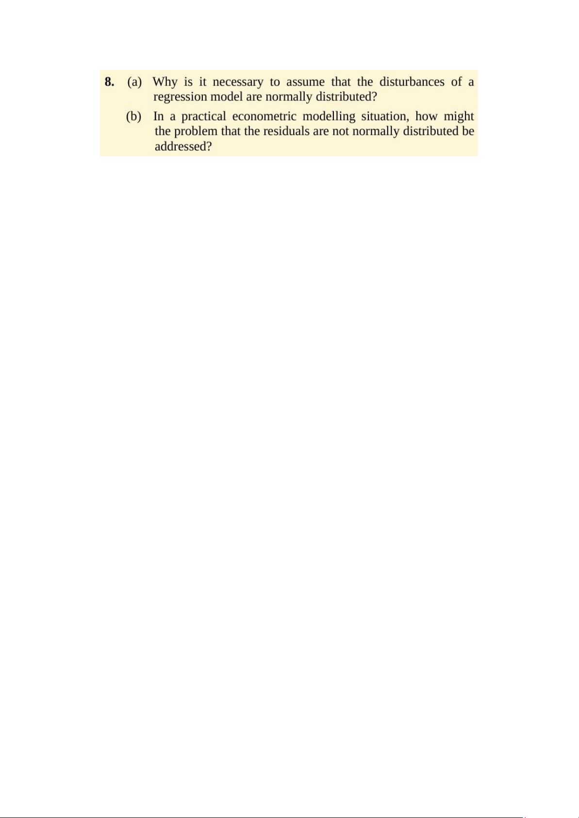
It is important to note that we did not need to assume normality in order to derive the
sample estimates of and or in calculating their standard errors. We needed the normality
assumption at the later stage when we come to test hypotheses about the regression coefficients,
either singly or jointly, so that the test statistics we calculate would indeed have the distribution
(t or F) that we said they would. b.
One solution would be to use a technique for estimation and inference which did not
require normality. But these techniques are often highly complex and also their properties are
not so well understood, so we do not know with such certainty how well the methods will
perform in different circumstances.
One pragmatic approach to failing the normality test is to plot the estimated residuals of the
model, and look for one or more very extreme outliers. These would be residuals that are much
“bigger” (either very big and positive, or very big and negative) than the rest. It is, fortunately
for us, often the case that one or two very extreme outliers will cause a violation of the
normality assumption. The reason that one or two extreme outliers can cause a violation of the
normality assumption is that they would lead the (absolute value of the) skewness and / or
kurtosis estimates to be very large.
Once we spot a few extreme residuals, we should look at the dates when these outliers occurred.
If we have a good theoretical reason for doing so, we can add in separate dummy variables for
big outliers caused by, for example, wars, changes of government, stock market crashes,
changes in market microstructure (e.g. the “big bang” of 1986). The effect of the dummy
variable is exactly the same as if we had removed the observation from the sample altogether
and estimated the regression on the remainder. If we only remove observations in this way, then
we make sure that we do not lose any useful pieces of information represented by sample points. lOMoAR cPSD| 58583460
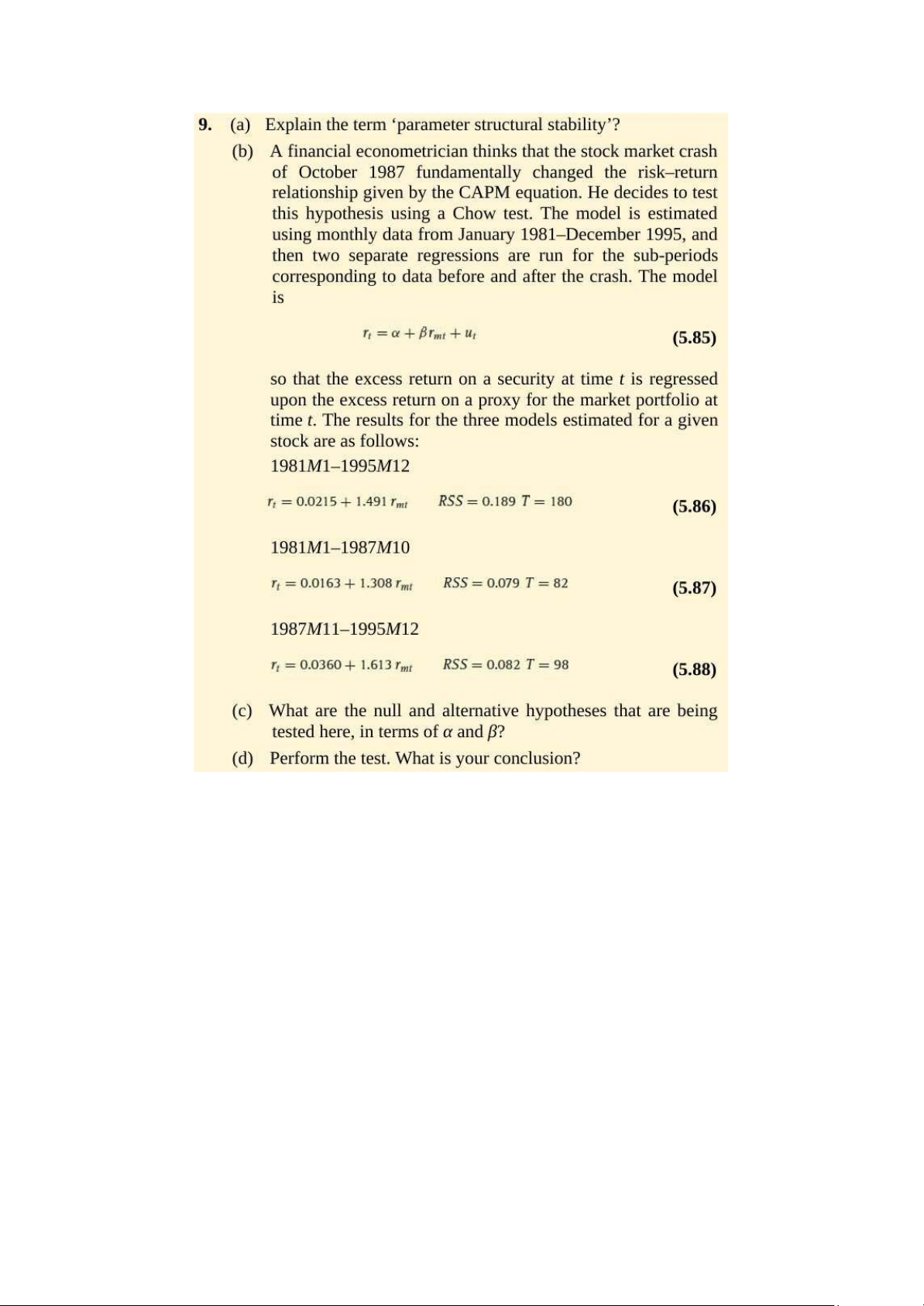
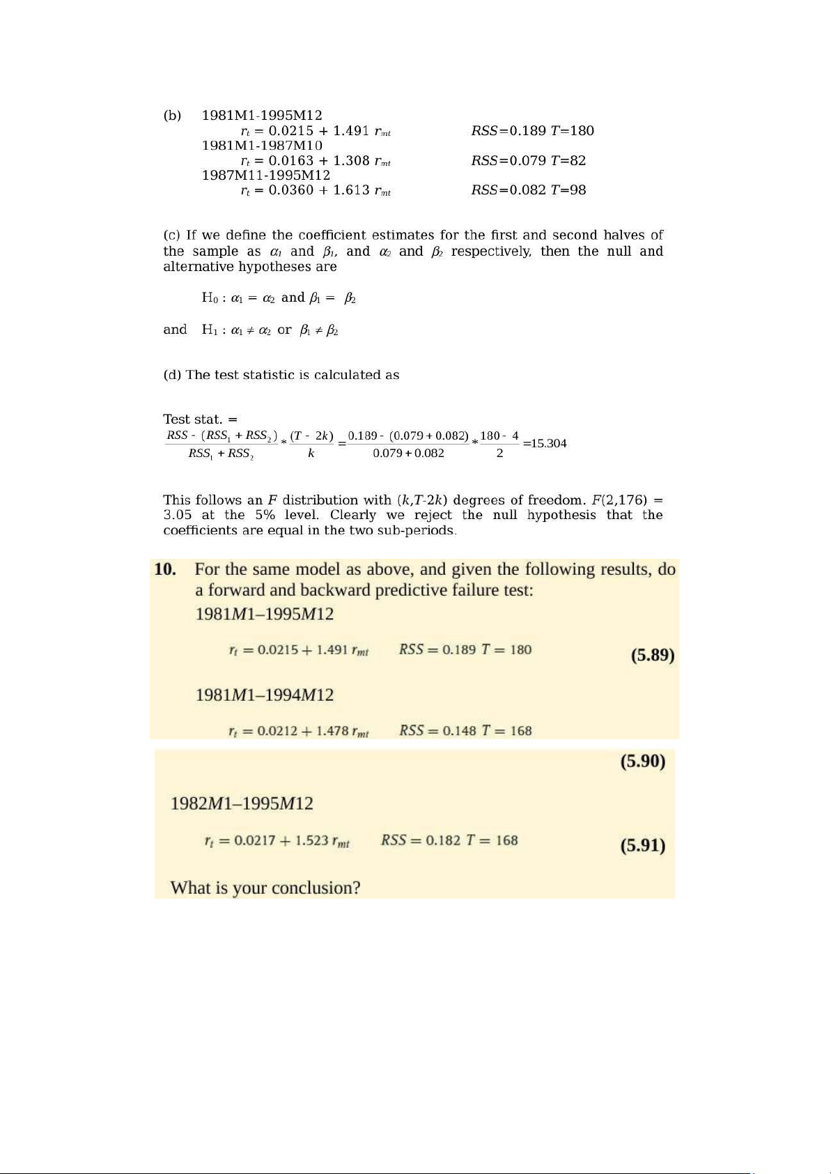
a. Parameter structural stability refers to whether the coefficient estimates for a regression
equation are stable over time. If the regression is not structurally stable, it implies that the
coefficient estimates would be different for some sub-samples of the data compared to others.
This is clearly not what we want to find since when we estimate a regression, we are implicitly
assuming that the regression parameters are constant over the entire sample period under consideration. lOMoAR cPSD| 58583460 lOMoAR cPSD| 58583460
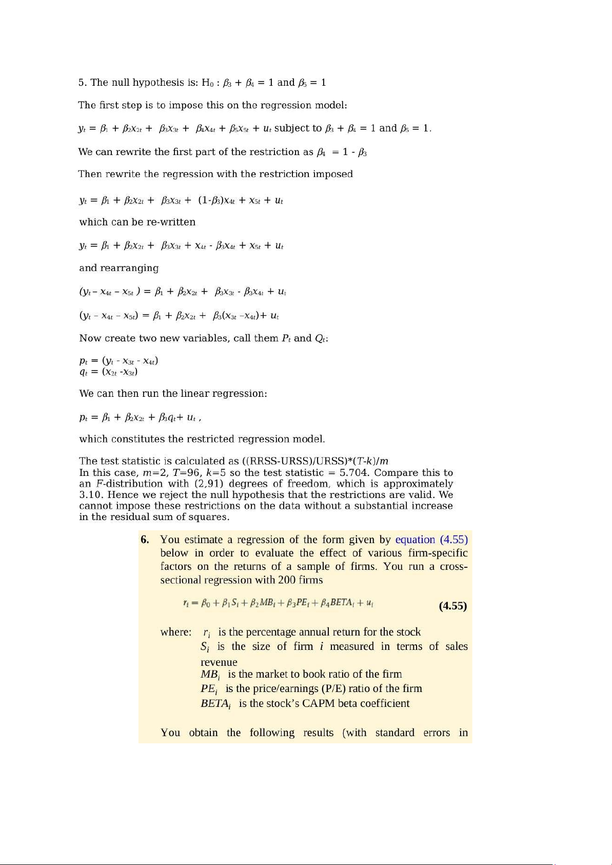
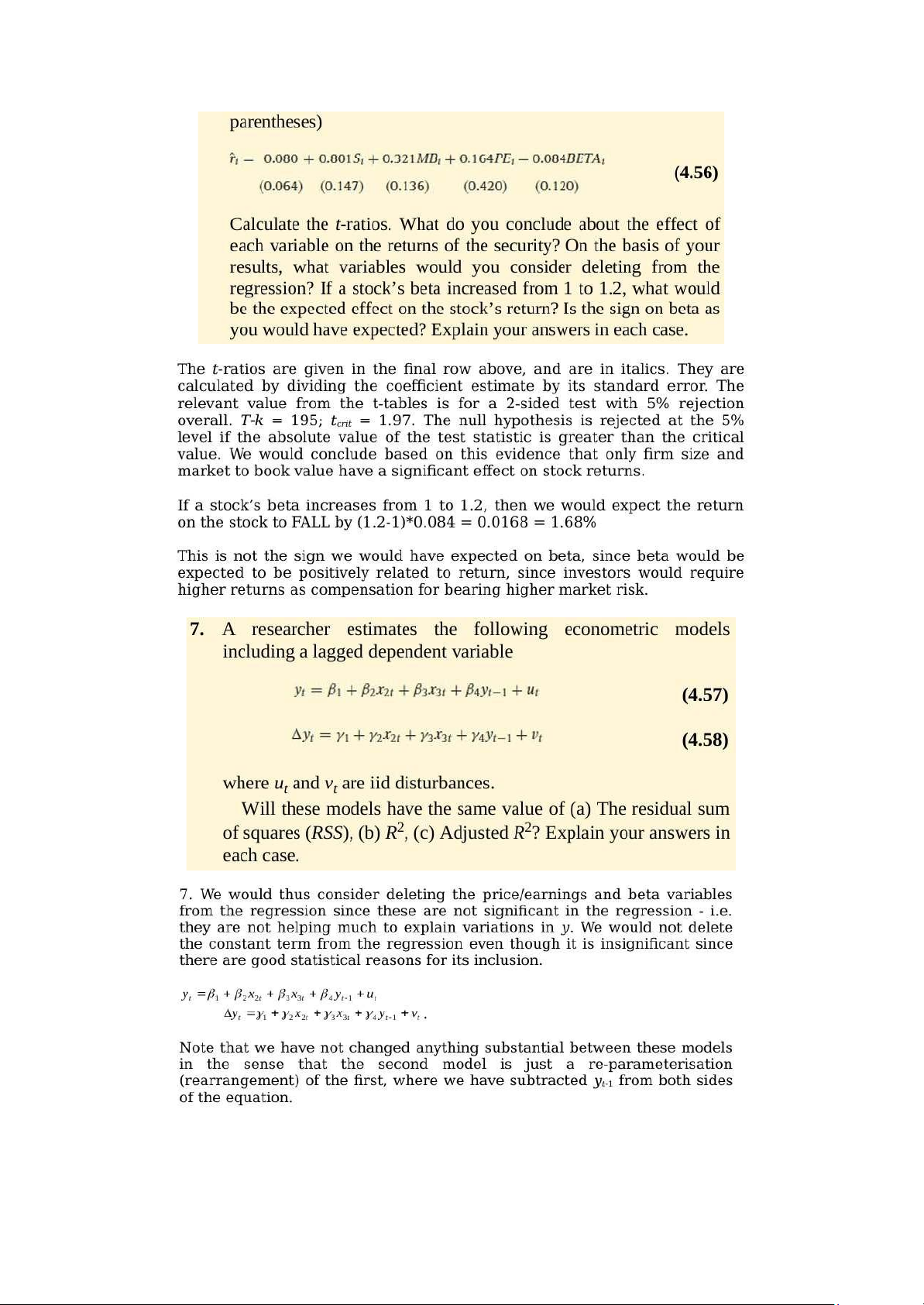
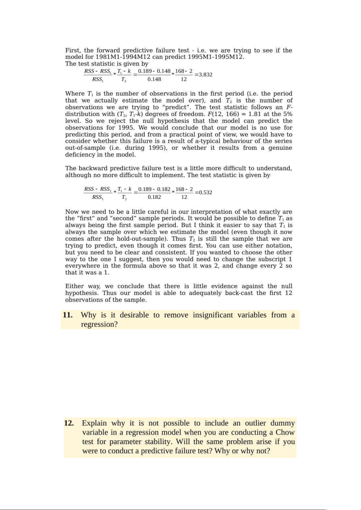
By definition, variables having associated parameters that are not significantly different from
zero are not, from a statistical perspective, helping to explain variations in the dependent
variable about its mean value. One could therefore argue that empirically, they serve no purpose
in the fitted regression model. But leaving such variables in the model will use up valuable
degrees of freedom, implying that the standard errors on all of the other parameters in the
regression model will be unnecessarily higher as a result. If the number of degrees of freedom
is relatively small, then saving a couple by deleting two variables with insignificant parameters
could be useful. On the other hand, if the number of degrees of freedom is already very large,
the impact of these additional irrelevant variables on the others is likely to be inconsequential. lOMoAR cPSD| 58583460
An outlier dummy variable will take the value one for one observation in the sample and zero
for all others. The Chow test involves splitting the sample into two parts. If we then try to run
the regression on both the sub parts but the model contains such an outlier dummy, then the
observations on that dummy will be zero everywhere for one of the regressions. For that sub-
sample, the outlier dummy would show perfect multicollinearity with the intercept and
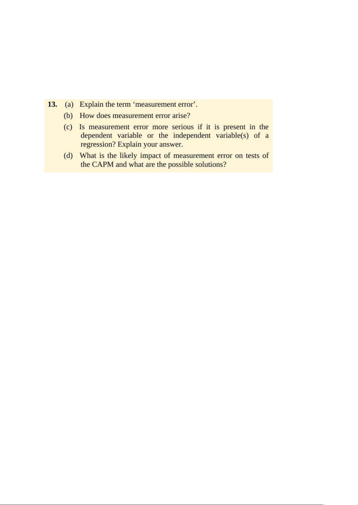
therefore the model could not be estimated. a) Measurement error:
Measurement error is the difference between the observed value of a Variable and
the true, but unobserved, value of that Variable.Measurement uncertainty is critical to
risk assessment and decision making. Organizations make decisions every day
based on reports containing quantitative measurement data. If measurement results
are not accurate, then decision risks increase. Selecting the wrong suppliers, could
result in poor product quality.
b) Measurement error arise due to Sources of systematic errors that may be
imperfect calibration of measurement instruments, changes in the environment
which interfere with the measurement process, and imperfect methods of
observation. A systematic error makes the measured value always smaller or
larger than the true value, but not both
c) Measurement is more serious when it is present in the independent variable of
regression.With multiple regression, matters are more complicated, as
measurement error in one variable can bias the estimates of the effects of other
independent variables in unpredictable directions. To “explain” something means
to give reasons why something is the case rather than something else.
d)The linear relationship between the return required on an investment (whether in
stock market securities or in business operations) and its systematic risk is
represented by the CAPM formula, which is given in the Formulae Sheet:
E(ri) = Rf + Bi(E(rm) - Rf)
E(ri) = return required on financial asset i Rf
= risk-free rate of return ßi beta value for lOMoAR cPSD| 58583460
financial asset i Bi E(rm) = average return on the capital market
we examine the effects of errors in measurement of the two independent variables,
return on market (Rm) and return on risk-free assets (Rf), in the traditional one-factor
capital asset pricing model (CAPM). After discussing Sharpe-Lintner's CAPM and
both Jensen and Fama's specifications thereof, we review briefly the recent results of
Friend and Blume , hereafter FB; Black, Jensen and Scholes ,hereafter BJS; and
Miller and Scholes ,hereafter MS. In Section II, we first explore possible sources of
measurement errors for both Rm and Rf; then we specify these errors
mathematically and derive analytically their effects on estimates of systematic risk of
a security or portfolio, , and the Jensen's measure of performance, . In Section III, we
derive an analytical expression for the regression coefficient of estimated b's where
we estimate the equation . The result is then examined to find the conditions under
which errors in measurement of Rm and Rf can cause b to have a positive or
negative value even if the true b is zero. The conditions are then used to examine
FB's results and their interpretation. In Section IV, an alternative hypothesis testing
procedure for the CAPM is examined. We show that the empirical results so derived
are also affected by the measurement errors and the sample variation of the
systematic risk. The relative advantage between the two different testing hypothesis
procedures is then explored. Finally, we comment on the relevance of the result to
the popular zero-beta model and indicate areas for further research.
Chap 6: Univariate Time-Series Modelling and Forecasting -
AR models use past values of the time series to predict future values, while MA models use past error terms. -
AR models capture the autocorrelation in a time series, while MA models capture the
moving average of the error terms. -
AR models can exhibit long-term dependencies in the data, while MA models are more
focused on capturing short-term fluctuations. -
AR models are suitable for data with trends, while MA models are useful for capturing
sudden shocks or irregularities in the data.
In practice, ARMA (autoregressive moving average) models combine both autoregressive and
moving average components to better capture the characteristics of time series data. lOMoAR cPSD| 58583460
ARMA models are of particular use for financial series due to their flexibility. They are fairly
simple to estimate, can often produce reasonable forecasts, and most importantly, they require
no knowledge of any structural variables that might be required for more “traditional” econometric analysis.
AR (Autoregressive) models are where the value of a variable in a time series is a function of
its own previous values (lagged values). It is useful for observing the momentum and mean
reversion effects. eg: stock prices
MA (moving average) models involve time series models where the value of a variable is a
function of the value of the error terms (both contemporaneous and past error terms). It captures
the effect of unexpected events eg: earnings surprise, covid-19 shock
ARMA models combine the AR and MA models and capture both mean reversion and shock
effects. Since financial time series is observed to have momentum and very volatile to shocks, ARMA models are useful lOMoAR cPSD| 58583460 a.
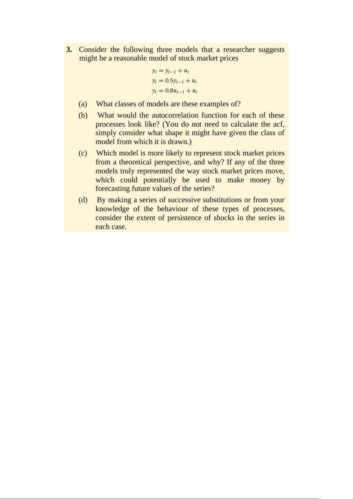
The first equation is a random walk or root process function, i.e. a non-stationary process with a value of 1.
The second equation describes a stationary Autoregressive cycle, since the coefficient is less than 1.
The third equation is a Moving Average model since its residual term is a number. b.
In the first equation, the non-stationary cycle will be fitted with a non decreasing ACF,
with correlation bars equal to 1.
ACF will decline very quickly during the second stationary phase, and its coefficients will
decrease by half the value of the last period.
At the first order on the horizontal axis, the third cycle would be non-zero because the MA's
ACF determines the order of the cycle. c.
While these processes are quite simplistic, the closest to any stock market process will
be a self-reliance process, as stocks are based on previous values, which are improved in the
form of residual acoustics. To say that a stock is a random march would mean that it is
completely unpredictable, except that this is not so in the longer term. The second method of
these three can be used to predict potential stock prices. But a real-world ARIMA (p, d, q)
model is typically suitable as a combination of the properties of the given processes to forecast future stock market values. lOMoAR cPSD| 58583460 d.
By the lagging time coefficient, we can say the persistence of a cycle. Persistence is
supreme in the first process, i.e. the process at a time t has been extremely persistent or relies
entirely on its importance across periods (t-1). The second cycle is less stable because it relies
partly on the importance of its previous era. In this cycle, persistence is lower. The continuity
with its last error term is high in the third MA cycle, because the coefficient is near 1.
a. Box and Jenkins were the first to consider ARMA modeling in this logical and coherent
fashion. Their methodology consists of 3 steps: -
Identification - determining the appropriate order of the model using graphical
procedures (e.g. plots of autocorrelation functions). -
Estimation - of the parameters of the model of size given in the first stage.This can be
done using least squares or maximum likelihood, depending on the model. -
Diagnostic checking - this step is to ensure thot the model actually estimated is
“adequate”. B & J suggest two methods for achieving this:
+ Overfitting, which involves deliberately fitting a model larger than that suggested
in step 1 and testing the hypothesis that all the additional coefficients can jointly be set to zero.
+ Residual diagnostics. If the model estimated is a good description of the data, there should
be no further linear dependence in the residuals of the estimated model. Therefore,
we could calculate the residuals from the estimated model, and use the Ljung-
Box test on them, or calculate their ocf. Ifeither of these reveal evidence of additional
structure, then we assume that the estimated model is not an adequate description of the data.
If the model appears to be adequate, then it can be used for policy analysis and for constructing
forecosts. If it is not adequate, then we must go bock tostoge 1 and tell the story again! b.
The main problem with the B & J methodology is the inexactness of the identification
stoge. Autocorrelation functions and portal autocorrelations for actual data are very difficult
to interpret accurately, rendering the whole procedure often little more than educated
guesswork. A further problem concerns the diagnostic checking storage, which will only
indicate when the proposed model is “too small” and would not inform on when the model proposed is “too large”. c.
We could use Akoike’s or Schwarz's Bayesian information criterion. Our
Objective would then be to fit the model order thot minimizes these.We can calculate the
volume of Akoike’s (AIC) and Schwarz's (SBIC) Boyesioninformotion criteria using the following respective formula