Giáo trình toán cao cấp 2 | trường Đại học Kinh tế Thành phố Hồ Chí Minh

lOMoAR cPSD| 47207194 lOMoAR cPSD| 47207194 FOREIGN TRADE UNIVERSITY PhD. DANG LE QUANG Lecture note ADVANCEDMATH2 Ho Chi Minh city - 2022 lOMoAR cPSD| 47207194 Mục lục
1. APPLICATIONS OF FUNCTIONS OF ONE VARIABLE IN ECO-
NOMICS ........................................................... 4
1.1. Review of single variable calculus .................................... 4
1.1.1. Some basics of functions of one variable.................................. 4
1.1.2. Limit of a function....................................................... 8
1.1.3. Derivative .............................................................. 10
1.2. Introduction to functions of one variable in economics .............. 12
1.3. applications of number sequences .................................. 14
1.3.1. Geometric sequence..................................................... 14
1.3.2. Applications in financial analysis........................................ 14
1.4. Applications of continuity in mathematics and in economics ........ 17
1.5. Applications of derivatives in economic analysis..................... 18
1.5.1. Derivatives and Marginal Values ........................................ 18
1.5.2. Elasticity Coefficient.................................................... 19
1.5.3. Law of diminishing marginal utility ..................................... 19
1.5.4. Average cost function, relationship between average cost function and marginal
function....................................................................... 20
1.5.5. Extreme values of economic function of one variable..................... 21
1.6. Applications of integral calculus in economic analysis .............. 24
1.6.1. Some integral expressions............................................... 24
1.6.2. Basic integral formulas.................................................. 24
1.6.3. Find total cost from marginal cost ...................................... 25
1.6.4. Exercises about finding surplus ......................................... 27
2. Some open problems on functional analysis (in one variable) . 29
2.1. The Theorem of Differentiable Functions ........................... 29 2 lOMoAR cPSD| 47207194 ADVANCED MATH 2
PhD. Đặng Lê Quang. Tel. 0764060787
2.2. Eliminating the indeterminate form using l’Hospital ................ 31
2.2.1. Multiplication indeterminate form (Zero Times Infinity)................. 32
2.2.2. Subtraction indeterminate form (Infinity Minus Infinity). ............... 32
2.2.3. Power infinity indeterminate form....................................... 33
2.3. Taylor’s series...................................................... 35
2.4. Improper integral................................................... 36 2.4.1. The properties of
convergence and divergence ........................... 36
TÀI LIỆU THAM KHẢO ....................................... 39 lOMoAR cPSD| 47207194 Chương1 APPLICATIONS OF FUNCTIONS OF ONE VARIABLE IN ECONOMICS
1.1. Review of single variable calculus
1.1.1. Some basics of functions of one variable
Definition 1.1. Let X,Y be subsets of R. Function f : X → Y is called a function of one
variable. The set X is called the domain of f, and is denoted by Df,the set of destination
of the function f, f(X), is called the range of f. A function, its domain, and its range, are declared by the notation:
f :X → Y
x 7→ f(x) = y
Or y = f(x), which provides us a way to return the value of the function f at an element
x, x is called a independent variable and y = f(x) is the value of the function at x. If f is
determined by a expression without any explanation is given then it automatically
means the domain of the function is a set of all the elements x such that the expression is defined.
Example 1.1. Find the domains of these following functions:
a. Suppose y = √9 − x2. Its domain is D = [−3,3]. 4
b. Suppose y = cos(x). Its domain is D = R. c. Suppose
. The expression is defined if 10 − x > 0 and x −
2 > 0. So, its domain is− D = (2,10). ⋆ Function composition lOMoAR cPSD| 47207194 ADVANCED MATH 2
PhD. Đặng Lê Quang. Tel. 0764060787
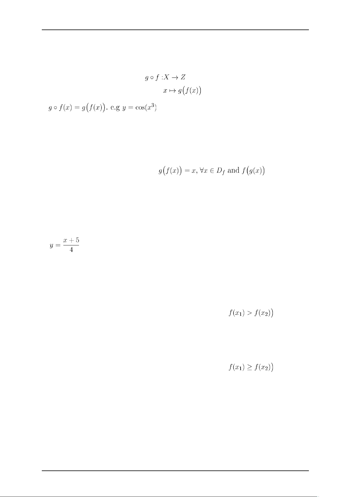
Let X,Y,Z be subsets of R. If function f from X to Y f : X → Y and function g : Y → Z,
"function composition" of f, g denoted by g ◦ f is a function such that: or
is the function composition of y = cos(u) and u = x3. ⋆ Inverse function
Suppose X,Y ⊂ R and the function f : X → Y is a bijection. Then, the function f(x) has
an inverse function g : Y → X such that ,
∀x ∈ Dg. We denote the inverse function of f(x) as f−1(x).
Example 1.2. Find the inverse functions of these following functions:
a. The inverse function of y = ex is y = ln(x). inverse function of y = 4x − 5 is . ⋆ Monotonic function
Let X,Y be subsets of R. The function f : X → Y is called strictly increasing (or strictly
decreasing) on X if for all x1,x2 ∈ X:
x1 < x2 (hoặc x1 > x2) ⇒ f(x1) < f(x2) hoặc
We call a function f(x) is monotonically increasing or monotonically decreasing on X if
for all x1,x2 ∈ X:
x1 ≤ x2 (hoặc x1 ≥ x2) ⇒ f(x1) ≤ f(x2) hoặc
In general, a function, which is either entirely non-increasing or non-decreasing, is
called a monotonic function. The term monotonic gives us an illustration of the image
of the graph of a function on its domain X: the graph of a increasing (decreasing)
function goes up (goes down) from the left to the right.
Example 1.3. Find the intervals in which the following functions are increasing or decreasing in their domains:
CHƯƠNG 1. APPLICATIONS OF FUNCTIONS OF ONE VARIABLE IN 5 ECONOMICS lOMoAR cPSD| 47207194 ADVANCED MATH 2
PhD. Đặng Lê Quang. Tel. 0764060787
a. f(x) = x is strictly increasing on R.
b. f(x) = cos(x) is strictly increasing on the interval (−π + k2π,k2π) and strictly decreasing
on the interval (k2π,π + k2π). ⋆ Bounded function:
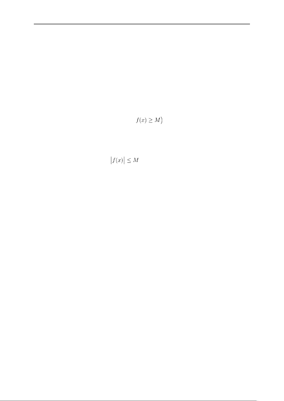
Let X,Y be subsets of R. A function f : X → Y is bounded above or below in X ⊂ R if
there exists a number M such that:
f(x) ≤ M hoặc
for all x ∈ X
If a function f(x) is either bounded above or bounded below on X, we says f(x) is
bounded on X. In other words, the function f(x) is bounded on X if there exists a positive
numberM such thatfor all x ∈ X.
Example 1.4. Consider these following functions:
a. the function y = sin(x)is bounded above R since −1 ≤ sin(x) ≤ 1. function y = x2 is
bounded below since x2 is always greater or equal to 0 for all x ∈ R.
⋆ Odd function and even function:
We call a set X ⊂ R symmetrical if for all x ∈ X we have −x ∈ X.
• a function f(x), which is defined on a symmetrical set X, is called a even function if
for all x ∈ X we have f(−x) = f(x). e.g y = x4, y = cos(x), y = |x| are even functions. The
graph of a even function is unchanged under reflection in the y-axis.
• a function f(x), which is defined on a symmetrical set X, is called a odd function if
forr all x ∈ X we have f(−x) = −f(x). e.g y = x3, y = sin(x) are odd functions. The graph
of an odd function will be symmetrical about the origin.
⋆ some of the most commonly used functions
1. Power function: y = xα (α ∈ R,α ̸= 0). The domain of this function depends on α.
• when α is a positive integer, D = R.
• when α is a negative integer, D = R \ {0}.
CHƯƠNG 1. APPLICATIONS OF FUNCTIONS OF ONE VARIABLE IN 6 ECONOMICS lOMoAR cPSD| 47207194 ADVANCED MATH 2
PhD. Đặng Lê Quang. Tel. 0764060787
• when α is a positive non-integer, D = [0,+∞).
• when α is a negative non-integer D = (0,+∞).
the function is strictly increasing if α > 0 and strictly decreasing if α < 0. the graph of
this function always passes through the point (1,1).
2. Exponential function: y = ax (a > 0,a = 1)̸ . The domain of a exponential function is D
= R and the range is (0,+∞). The function is increasing if a > 1 and is decreasing if 0 <
a < 1. The graph of this function always passes through the point (0,1). The graph
always lies above the x-axis and has the x-axis as a horizontal asymptote.
3. Logarithmic function: y = loga(x) (a > 0,a = 1)̸ . The domain is D = (0,+∞) and its inverse
function is y = ax. The graph of the logarithmic function and the graph of the
exponential function are reflection of each other in the line y = x.
The function is increasing when a > 1 and is decreasing when 0 < a < 1. 4. Trigonometric functions:
• The functions y = sin(x); y = cos(x) have the domains defined as D = R,and their
range are [−1,1], they are periodic with period 2π.
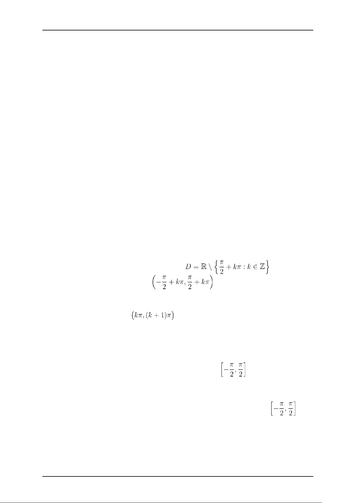
• The function y = tan(x) has the domain and the range
R, it is strictly increasing on
, and is periodic with period π.
• The function y = cot(x) has the domain D = R \ {kπ : k ∈ Z},and the range R, it is strictly increasing on
, and is periodic with period π.
⋆ Inverse trigonometric functions:
1. The function y = arcsin(x).
• The function y = sin(x) is strictly increasing on therefore its inverse
function is x = arcsin(y). x denotes the independent variable and y denotes the
dependent variable, then the inverse function is denoted by y = arcsin(x).
• The function y = arcsin(x) has the domain D = [−1,1] and the range .
Moreover, its inverse function y = arcsin(x) is an odd and increasing function. 2.
The function y = arccos(x).
• The inverse function of y = cos(x) on the interval [0,π] is denoted by y = arccos(x).
CHƯƠNG 1. APPLICATIONS OF FUNCTIONS OF ONE VARIABLE IN 7 ECONOMICS lOMoAR cPSD| 47207194 ADVANCED MATH 2
PhD. Đặng Lê Quang. Tel. 0764060787
• The function y = arccos(x) has the domain D = [−1,1], and the range [0,π].
Moreover, the function y = arccos(x) is a decreasing function.
3. The function y = arctan(x).
• The function y = arctan(x) is inverse function of the function y = tan(x) on .
• The function y = arctan(x) has the domain D = R, and the range .
Moreover, the function y = arctan(x) is an odd and increasing function.
4. The function y = arccot(x).
• The function y = arccot(x) is the inverse function of y = cot(x) trong (0,π).
• the function y = arccot(x) has the domain D = R, and the range (0,π).
Morover y = arccot(x) is a decreasing function.
5. In general, Power functions, exponential functions, logarithmic functions,
trigonometric functions and inverse trigonometric functions are called basic
elementary functions. From elementary functions, by adding subtracting,
multiplying or dividing a finite number of any of the previous functions we construct
more complex functions which are called elementary functions . 1.1.2. Limit of a function
Definition 1.2. A function f is continuous at a if:
lim f(x) = f(a) x→a
notice that the the terminology (1.2) requires 3 criteria in order to obtain the
continuous of f at a:
1. f(a) is defined (i.g a belongs with the domain of the function f).
2. lim f(x) exists. x→a
3. lim f(x) = f(a). x→a
Example 1.5. Find the sets of points where these following functions are discontinuous
CHƯƠNG 1. APPLICATIONS OF FUNCTIONS OF ONE VARIABLE IN 8 ECONOMICS lOMoAR cPSD| 47207194 ADVANCED MATH 2
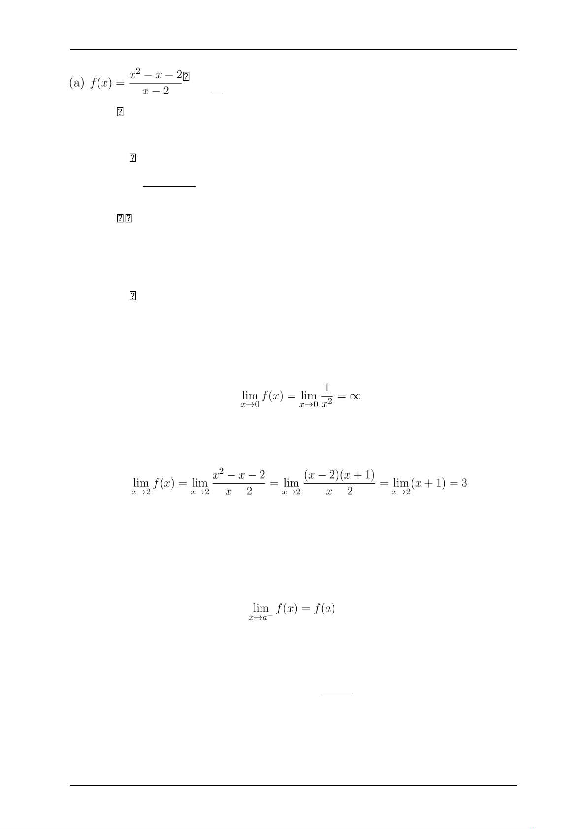
PhD. Đặng Lê Quang. Tel. 0764060787 1 if x = 0
(b) f(x) = x2 ̸ 1 if x = 0 x2 x − − (c) f(x) = x − 2 if x ̸= 2 if 1 x = 2 2 Solution
(a) Since f(2) is not defined, f is discontinuous at 2.
(b) Here, f(0) = 1 is defined but
So, f is discontinuous at 0. (c) We consider: − −
We see lim→ = 3 ̸= f(2) = 1 so f is discontinuous at 2. x 2
Definition 1.3. A function f is called continuous at a if:
lim f(x) = f(a) x→a+
and left continuous at a if:
Definition 1.4. A function f is called continuous on a interval if it is continuous at each point on that interval.
Example 1.6. Prove that the function f(x) = 1 − √1
− x2 is continuous in the interval [−1,1]. Solution
CHƯƠNG 1. APPLICATIONS OF FUNCTIONS OF ONE VARIABLE IN 9 ECONOMICS lOMoAR cPSD| 47207194 ADVANCED MATH 2
PhD. Đặng Lê Quang. Tel. 0764060787
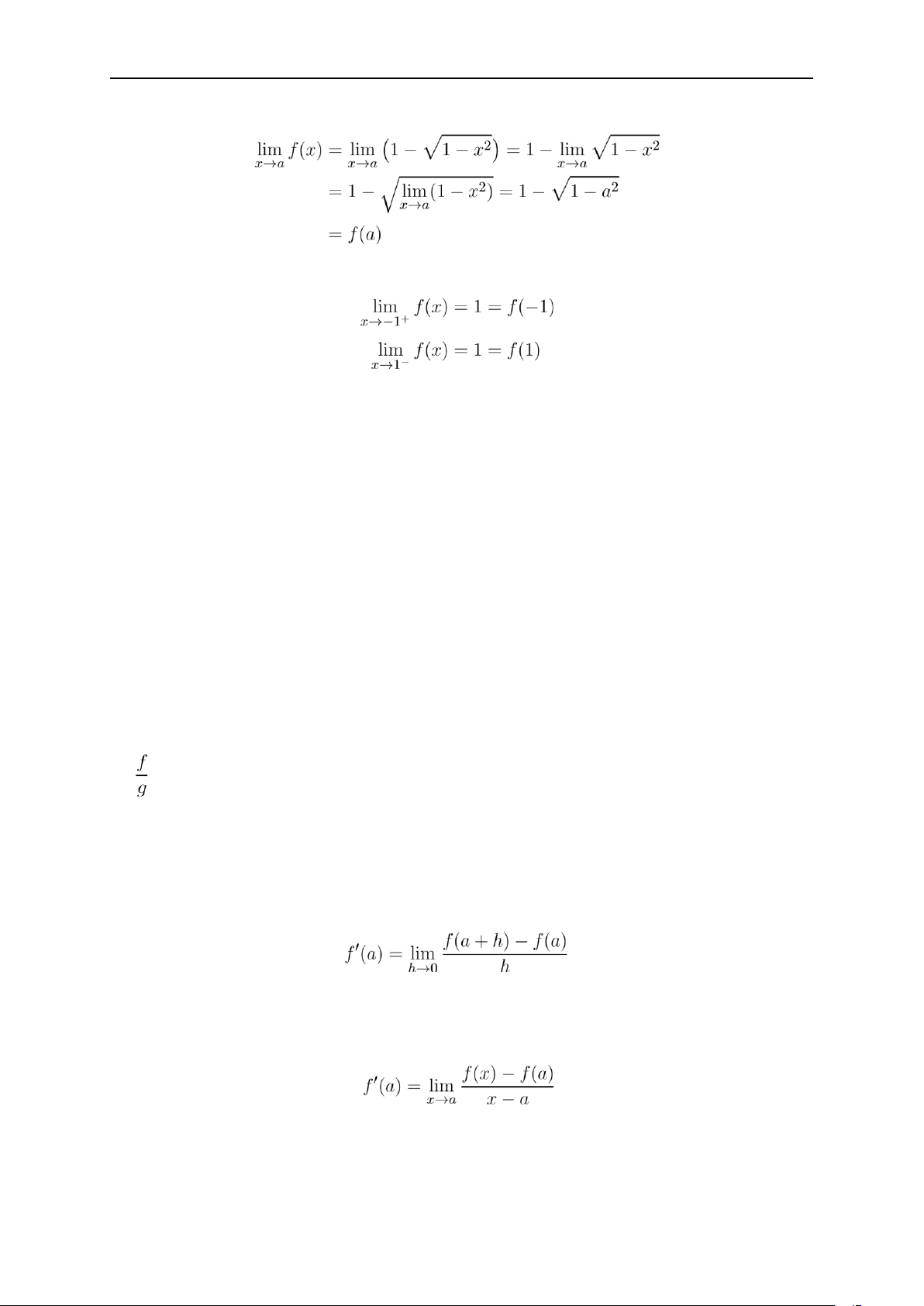
With −1 < a < 1, we have:
Consider 2 points at the edge, we have:
Therefore, f is right continuous at −1 and left continuous at 1. That leads to f is
continuous on [−1,1].
Theorem 1.1. If f and g are continuous at a and c which are constants, these following
functions are too continuous at a: 1. f + g 2. f − g 3. cf 4. fg
5. nếu g(a) ̸= 0 1.1.3. Derivative
Definition 1.5. Derivative of a function f at a denoted by f′(a) is :
If this limit exists, we write x = a + h. Then, h = x − a and h approaches 0 if and only if x
approaches a. Therefore, there is an equivalent definition of derivative as below: when the limit above exists.
Example 1.7. Find the derivative of f(x) = x2 − 8x + 9 at a.
CHƯƠNG 1. APPLICATIONS OF FUNCTIONS OF ONE VARIABLE IN 10 ECONOMICS lOMoAR cPSD| 47207194 ADVANCED MATH 2
PhD. Đặng Lê Quang. Tel. 0764060787 Solution
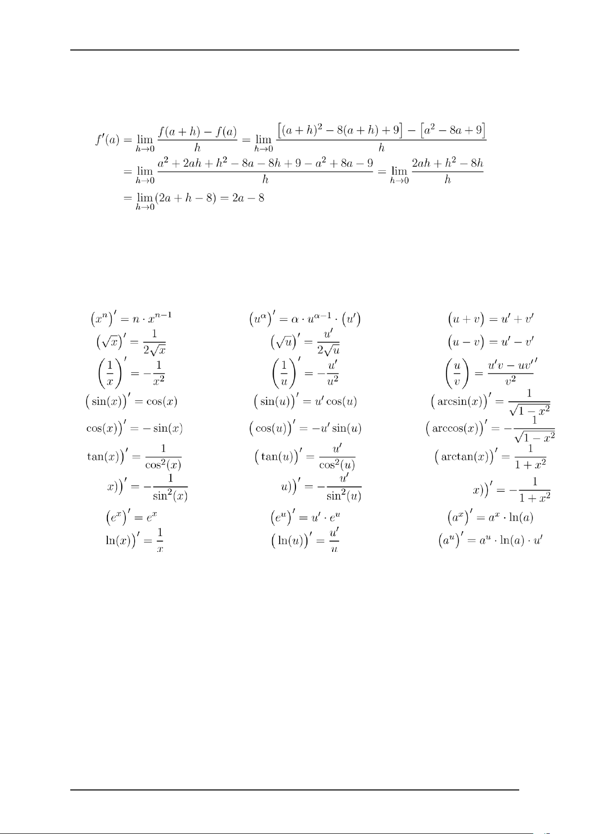
As definition of the derivative (1.5), we have:
Definition 1.6. The function is f differentiable at a if f′(a) exists. A function is
differentiable on an open interval (a,b) [or (a,∞) or (−∞,a) or (−∞,∞)] if it is
differentiable at every element on that interval.
Some of the general differentiation formulas cot( cot( arccot(
CHƯƠNG 1. APPLICATIONS OF FUNCTIONS OF ONE VARIABLE IN 11 ECONOMICS lOMoAR cPSD| 47207194 ADVANCED MATH 2
PhD. Đặng Lê Quang. Tel. 0764060787
1.2. Introduction to functions of one variable in economics
⋆ Supply function and demand function
The economists use terminologies supply functions and demand functions to shows
the functional relationship between quantity demanded and quantity supplied for a
commodity and its various determinants. That relationship depends on the price of the
commodities. The equation for supply function and demand function is of the forms as below:
• The supply function: QS = S(p) • The demand function: QD = D(p) where,
– p is the price of the commodity.
– QS is quantity supplied: which is the quantity of commodities that producers
are willing to sell at a particular price at a particular point of time.
– QD is quantity demanded: which is the quantity of commodities that
consumers are willing to purchase at a particular price at a particular point of time.
When we consider the model of the supply function, we construct a assumption
that all other factors are constants.
According to the law of market in economics for normal commodities, the supply
function is a increasing function and the demand function is decreasing function.
The graph of the supply function (demand function) is called the supply curve
(demand curve). The point at which the two curves intersect is the equilibrium market point.
• Watch out: In economics, there calls popularly the inverse
function of the function QS = S(p) the supply function and calls
the inverse of the function QD = D(p) the demand function.
QS = S(p) ⇔ p = S−1(QS)
QD = D(p) ⇔ p = D−1(QD)
⋆ Cost function???: is a function which shows the dependence of the total cost
(TC) on the quantity (Q): TC = TC(Q).
⋆ Revenue function is a function which shows the dependence of the total revenue
(TR) on the quantity (Q): TR = TR(Q).
CHƯƠNG 1. APPLICATIONS OF FUNCTIONS OF ONE VARIABLE IN 12 ECONOMICS lOMoAR cPSD| 47207194 ADVANCED MATH 2
PhD. Đặng Lê Quang. Tel. 0764060787
⋆ Profit function : is a function which shows the dependence of the total profit π
(TR) on the quantity (Q): π = π(Q).
The profit function can be found by π(Q) = TR(Q) − TC(Q).
⋆ Utility function (consumption function): The economist uses consumption
function to show the relationship between the consumption and the yields
(Y): C = C(Y ).
⋆ Saving function: is a function which shows the dependence of the savings
(S) on the yields (Y ): S = S(Y ).
⋆ Short-run production function
The economist uses the terminology production function to show the relationship
between the output (the total quantity of goods or services produced in a given
time period) of a producer and inputs, which is called Factors of
Production,examples of inputs include labor (workers’ time), fuel, materials,.. ... In
economics, the terminologies short-run and long-run are defined as follows
– the short run is generally defined as the time horizon over which at least one
factor of production are "sticky," or inflexible.
– The long run is a situation where all main factors of production are variable.
In analyzing production, economists are often interested in two important factors
of production: (Capital) and (Labour),which are denoted by K and L. For example,
the production function is in form of Cobb-Douglas depending on one of two
factors that is capital and labour: Q = aKα; Q = bKβ với a,b,α,β are positive numbers.
⋆ The investment function refers to investment -interest rate relationship: I = I(r),
where r = rate of interest.
⋆ Hàm quỹ vốn theo thời gian:??? K = K(t), where t = time.
⋆ The investment function refers to investment -time relationship:
I = I(t), where t = time.
1.3. applications of number sequences 1.3.1. Geometric sequence
Definition 1.7. A geometric progression, also known as a geometric sequence, is a
sequence (un) such that: un+1 = un·q, ∀n = 1,2,3,... with q is a constant. We call q the
common ratio. Moreover, when |q| < 1, the geometric sequence is also called the
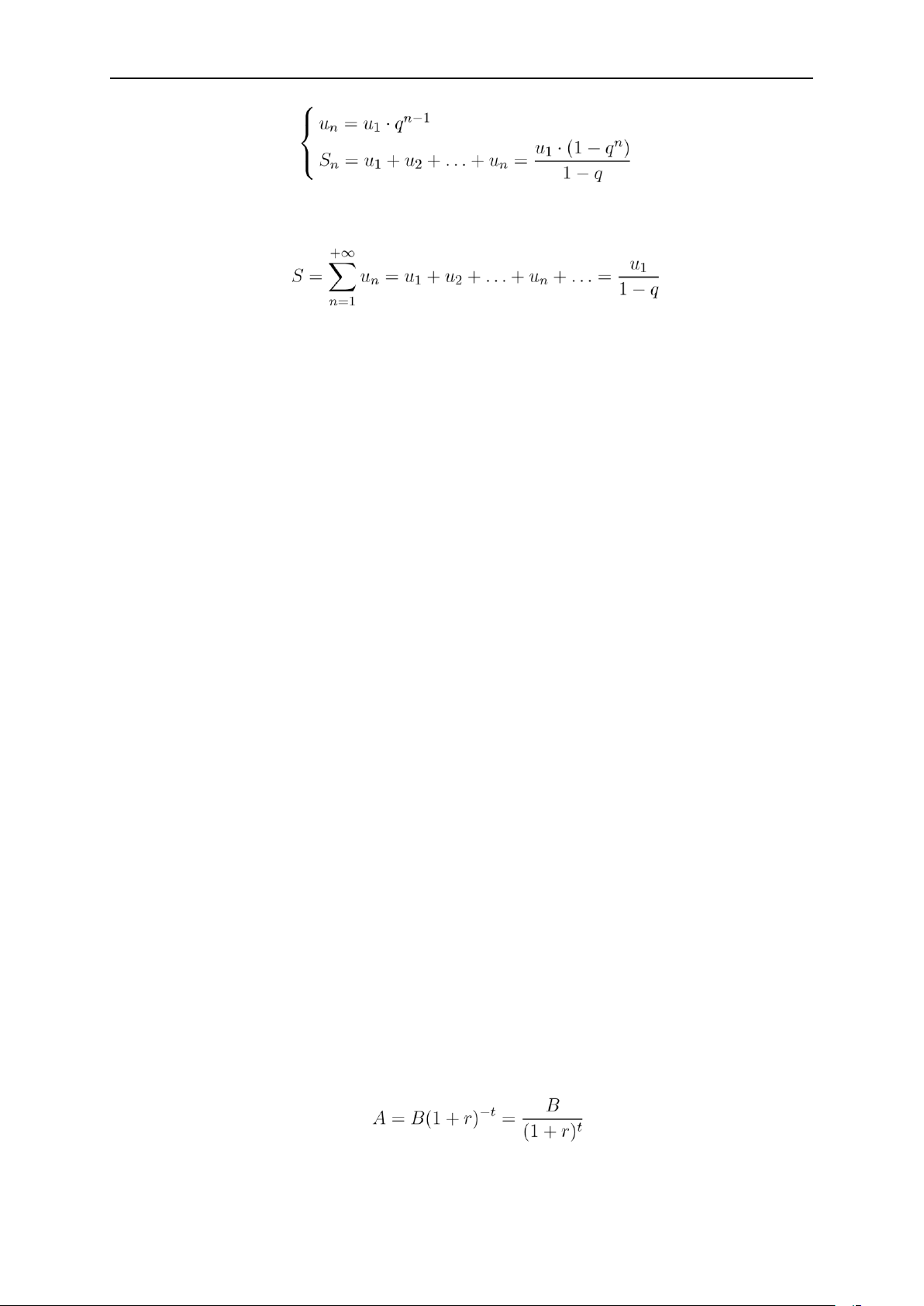
infinitely decreasing geometric sequence. We have these following formulas:
CHƯƠNG 1. APPLICATIONS OF FUNCTIONS OF ONE VARIABLE IN 13 ECONOMICS lOMoAR cPSD| 47207194 ADVANCED MATH 2
PhD. Đặng Lê Quang. Tel. 0764060787
When a geometric sequence is a infinitely decreasing geometric sequence, i.g |q| < 1,
1.3.2. Applications in financial analysis
a) Calculate present value and future value of money
Suppose a person has a sum of money A deposited in aa bank with a fixed rate of
interest.Then, After a period of time, that one will receive a larger amount of
money is B = A+ the interest .
That amount of money B is called the future value of the current asset A invested
today. A is called the present value of B that one will possess in the future.
In the money market, the rate of interest is viewed as the price of funds for get a
loan. Interest rates are regulated very differently. In economics, when one analyzes
financial activity, it is assumed that there is a common interest rate. We denote
the general interest rate by r.
Suppose a person has a sum of money A, then after one year, with the interest rate
per year is r, that person is going to have a lump sum of the interest and the principal is:
Bt = A + rA = (1 + r)A
Let Bt be the amount of money the person have after t years, we have a geometric
sequence with common ratio q = 1 + r. One has:
Bt = B0qt = A(1 + r)t
The future value of A that the person having today after t years is:
B = A(1 + r)t
The present value of B that the person obtaining after t years is:
CHƯƠNG 1. APPLICATIONS OF FUNCTIONS OF ONE VARIABLE IN 14 ECONOMICS lOMoAR cPSD| 47207194 ADVANCED MATH 2
PhD. Đặng Lê Quang. Tel. 0764060787
Example 1.8. An investment project requires a current cost of 200 million VND and
will bring in 300 million VND in 4 years. With interest rate is 6%, Evaluate whether
this project should take place? Solution
We have the future value of 200 million VND after 4 years is:
A = 200 · (1 + 0.06)4 ≈ 252,5 (million VND)
This amount is less than 300 million we will obtain, so the project should take place.
b) Ordinary Annuity and Capital flows
Ordinary Annuity An ordinary annuity is a series of equal payments made at the
end of consecutive periods over a fixed length of time. While the payments in an
ordinary annuity can be made as frequently as every week, in practice they are
generally made monthly, quarterly, semi-annually, or annually. An ordinary annuity
paid yearly is called an annuity.
Union dues and instalment payments, which are paid monthly or annually, are ordinary annuities.
By using the method for calculating the future value and present value as above
combined with the formula of the sum of a geometric sequence, we can calculate
the present value and future value of an ordinary annuity.
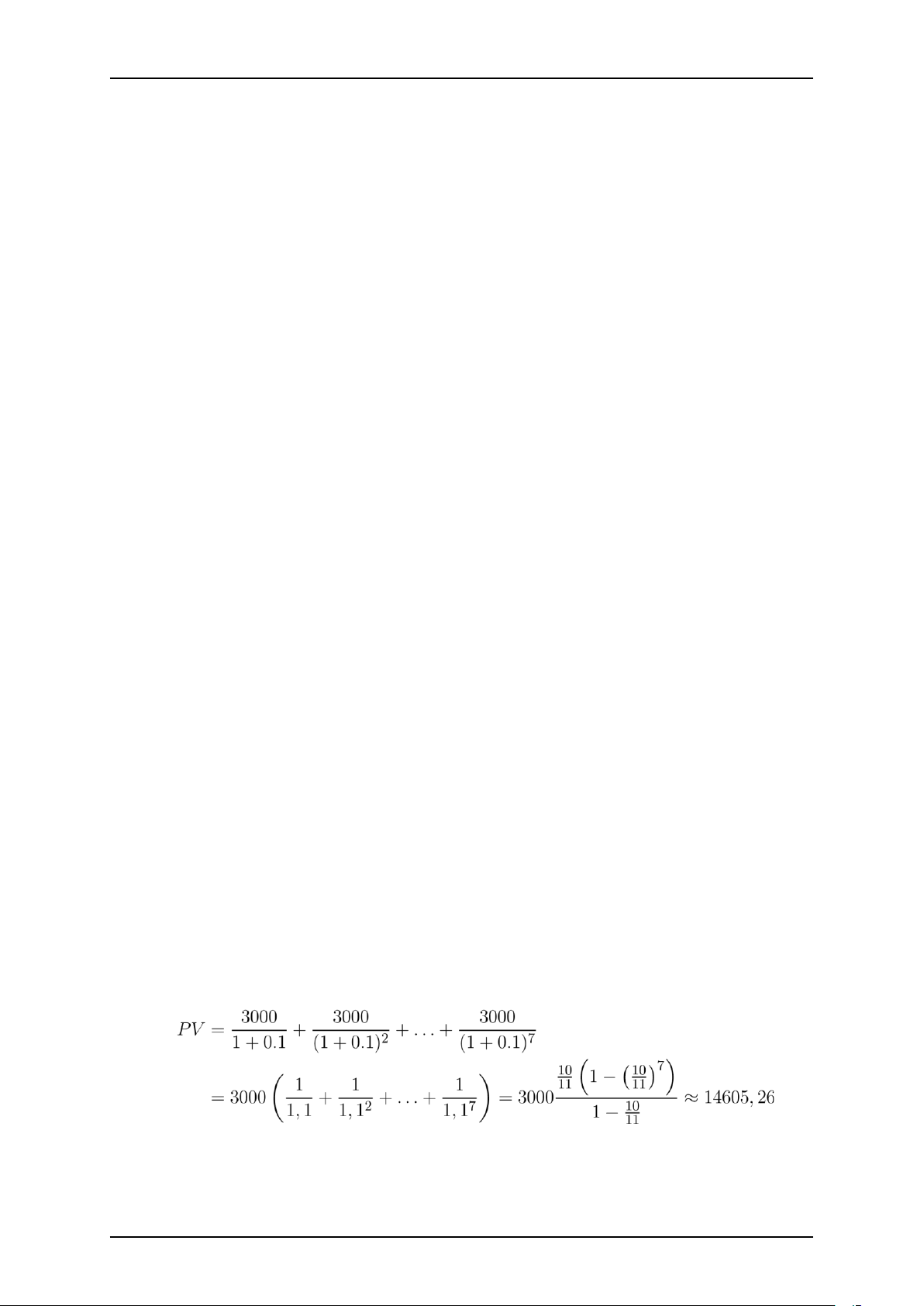
Example 1.9. An investment project after one year will bring you $3000 per year,
consecutively for the next 7 years. Ask that the capital flow must be initially
invested. How much can you accept that project if the annual interest rate is 10% ? Giải
The present value of cash flows is (PV):
So, the project just should take place if the original capital is less than $14605,26.
CHƯƠNG 1. APPLICATIONS OF FUNCTIONS OF ONE VARIABLE IN 15 ECONOMICS lOMoAR cPSD| 47207194 ADVANCED MATH 2
PhD. Đặng Lê Quang. Tel. 0764060787
Example 1.10. Suppose you intend to buy a car by making installment payments.
By this method, after one month from the time of receipt, you have to pay
regularly each month a certain amount of money, consecutively for 60 months.
Suppose the price of a motorcycle at the time you buy a car is $15000 and the
bank interest rate is 1%/month. With what is the monthly payment, is the
installment purchase acceptable? Solution
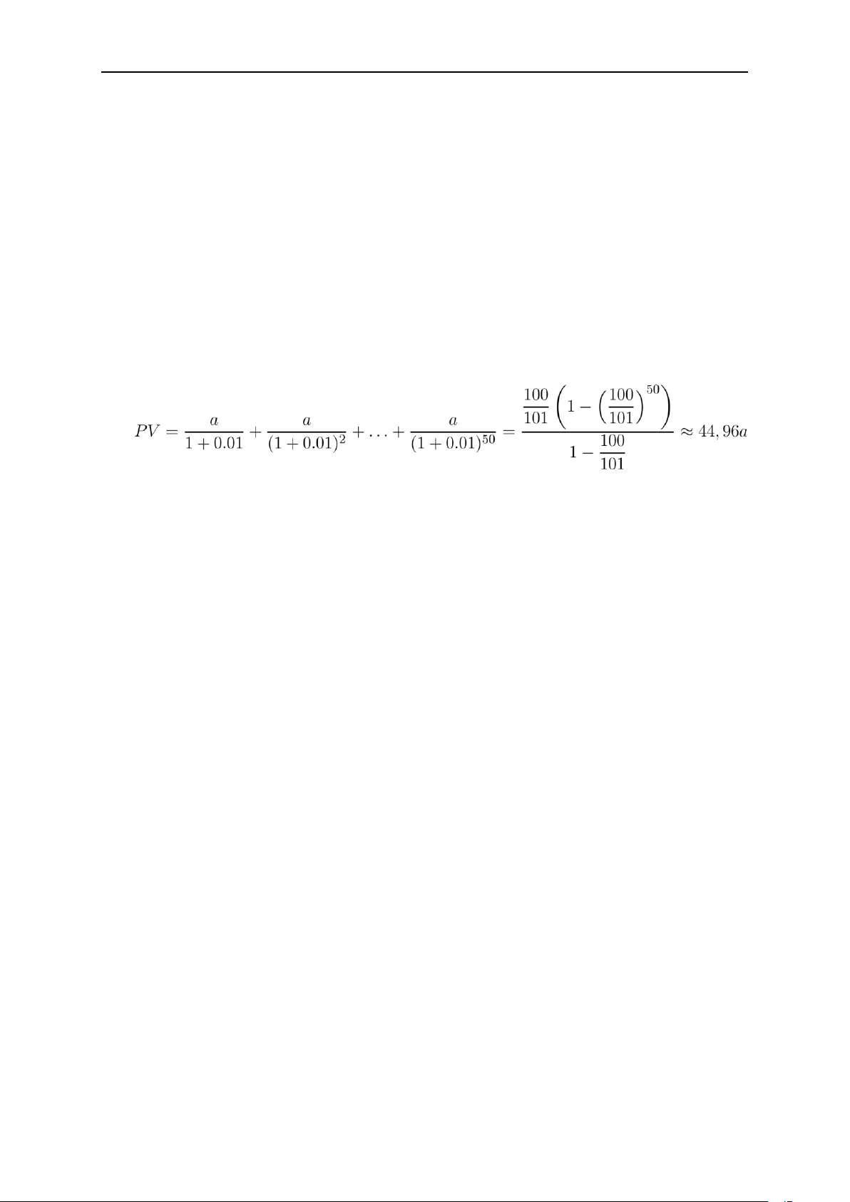
Suppose a monthly payment is a. The present value of the entire installment cash
flow at the time of receipt is:
The installment purchase will be equivalent to the purchase of immediate payment if:
PV = 49,96a = 15000 ⇔ a ≈ 300,24
1.4. Applications of continuity in mathematics and in economics ⋆ Weierstrass theorem
Theorem 1.2. If the function f(x) is continuous on the interval [a,b], then it reaches
its maximum and minimum values on the interval [a,b], i.g, there exist x1,x2 ∈ [a,b] , such that:
f (x1) = max f(x) và f (x2) = min f(x) x∈[a,b] x∈[a,b]
⋆ Intermediate value theorem
Theorem 1.3. Assume that f(x) is continuous on [a,b] and f(a) ≠ f(b). If you take on
any value c between f(a) and f(b) that is f(a)cf(b) or f(b)cf(a), there exists a x0 ∈ (a,b) such that
Corollary 1.1. If the function f(x) is continuous on [a,b] and f(a) · f(b) =
CHƯƠNG 1. APPLICATIONS OF FUNCTIONS OF ONE VARIABLE IN 16 ECONOMICS lOMoAR cPSD| 47207194 ADVANCED MATH 2
PhD. Đặng Lê Quang. Tel. 0764060787
0,then, there exists x0 ∈ (a,b) such that f(x0) = 0.i.g, the equation f(x) = 0 has at least one solution in (a,b).
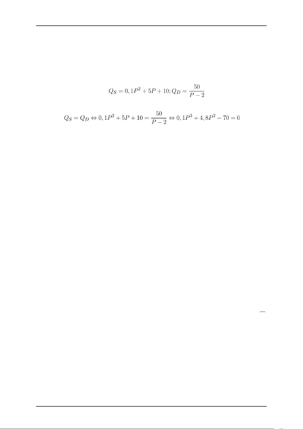
Example 1.11. The following equations describe the market equilibrium model QS = QD:
Prove that the above model has an equilibrium price on the interval (3,5). We have: (1.1)
Consider the function f(P) = 0.1P3 +4.8P2 −70 continuously on [3,5]. Because we
have f(3) · f(5) < 0 , the solution to the equation (1.1) is on the interval (3,5). It
follows that the above model has an equilibrium price on (3,5).
1.5. Applications of derivatives in economic analysis
1.5.1. Derivatives and Marginal Values
Given the function y = f(x) where x,y are economic variables, let x0 be a point in the
domain of the function. The following function:
My = f′(x)
is called Marginal function. The value of My at x0, My(x0),is called Marginal value
of f(x) at the element x0 ( or in short, marginal value at x0 ).
Interpretation: at x0, When x changes one unit , then the value of the function f(x)
changes a quantity approximately My(x0) = f′(x0).
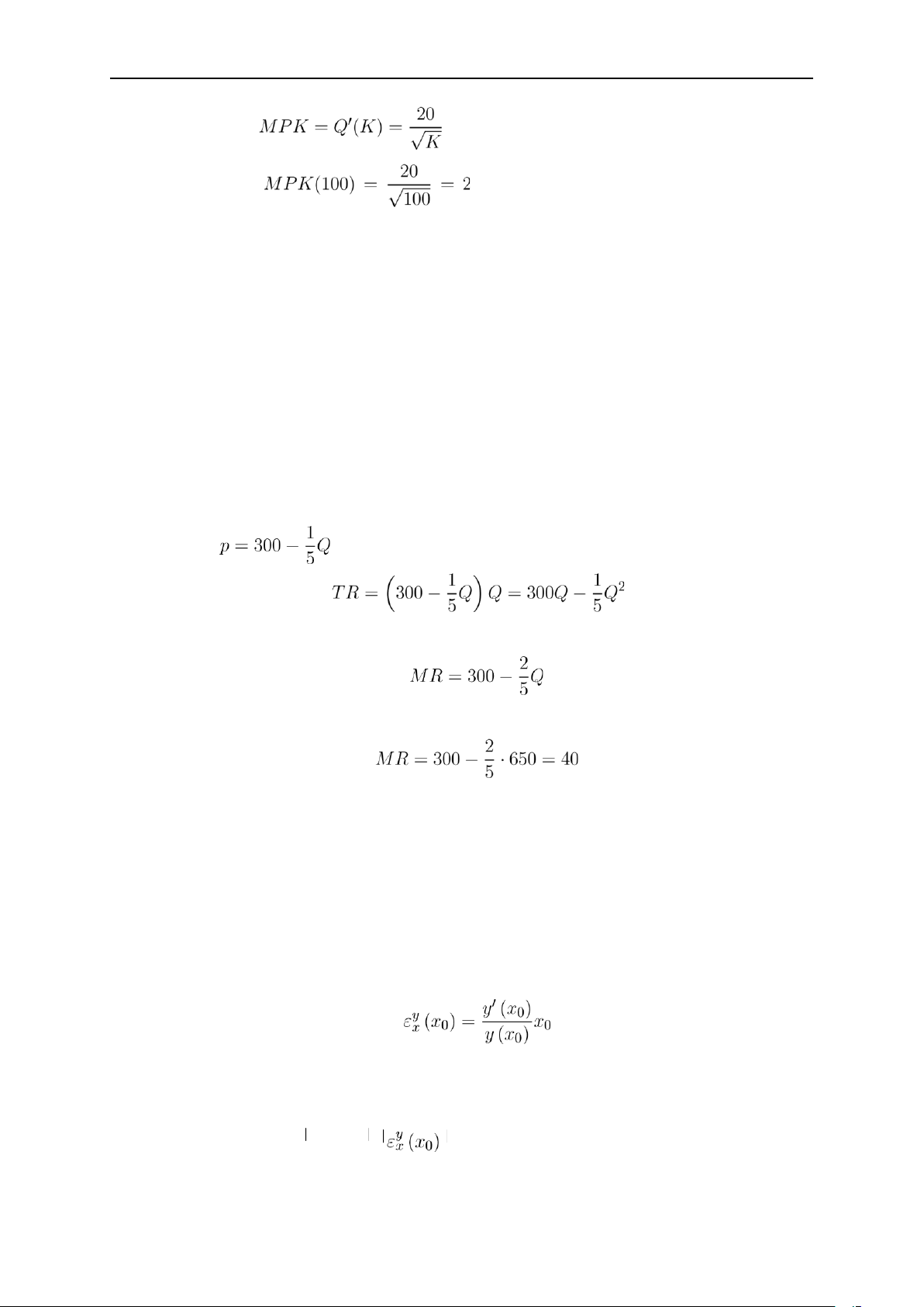
Example 1.12. Suppose the short run production function is given by Q = 40√K ; K > 0.
a. Find the marginal Product of Capital MPK = Q′(K).
b. At K0 = 100, if K is increased by one unit, how much will the units
produced by the company change? Solution
CHƯƠNG 1. APPLICATIONS OF FUNCTIONS OF ONE VARIABLE IN 17 ECONOMICS lOMoAR cPSD| 47207194 ADVANCED MATH 2
PhD. Đặng Lê Quang. Tel. 0764060787 a. We have: b. We have:
. So, K0 = 100. We can conclude that if K is
increased by one unit, the company can increase by 2 units of its production.
Example 1.13. A monopolist firm sells its products in the market with the demand function given by: Q = 1500 − 5p
Calculate marginal revenue at the quantity Q = 650 and interpret the result. Solution We have
. So, the revenue function is:
The marginal revenue function is calculated by:
At the quantity Q = 500, we have:
That means, at the quantity Q = 500, when one more unit is produced, the total
revenue of the company will increase by $40 1.5.2. Elasticity Coefficient
Given the function y = f(x) where x,y are economic variables, let x0 be an element
in the domain of the function. The following value
is called the Elasticity Coefficient of y expressed in terms of a variable x at x0.
Interpretation: At x0, when x changes by 1% ,the value of the function y = f(x) changes by about %.
Example 1.14. If the demand function is describe as Q = 1400 − p2, the elasticity
coefficient at the price p is:
CHƯƠNG 1. APPLICATIONS OF FUNCTIONS OF ONE VARIABLE IN 18 ECONOMICS