Lý thuyết chương 4: Some linear models used in economic | Môn toán cao cấp

lOMoAR cPSD| 49519085
Lecturer: Nguyen Duong Nguyen, Mathematics Department, Faculty of Basic Science, FTU
Chapter 4. SOME LINEAR MODELS USED IN ECONOMIC ANALYSIS
4.1. Leontief Input – Output Model
The Leontief Input - Output model refers to the determination of the total demand
for products of each manufacturing industry in the overall economy.
Consider an economy with n manufacturing industries (sectors): industry 1, industry
2, industry 3, ..., industry n.
The total demand for products of industry i (i = 1, 2, 3, ...) includes: -
Demand from industries in the economy (including industry i) using the
products of industry i for their production process, is called intermediate demand. -
Demand from the users of the product of industry i for consumption or export, is called final demand.
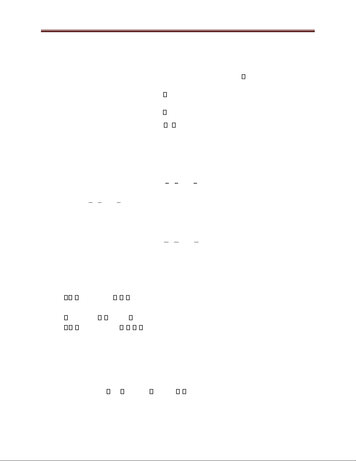
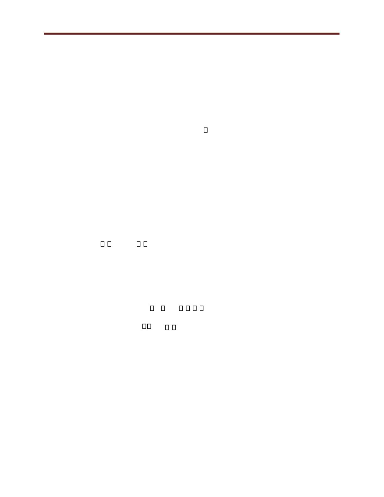
The total demand for products of industry i (i = 1, 2, ..., n) is denoted xi and is determined as follows: x i xi1 x i2 xin b i
where xik is the product value of industry i that industry k needs to use for its production (intermediate demand).
bi is the product value of industry i needed for consumption and export demand (final demand)
The above formula can be written as: x xi1 xi2 i .x1
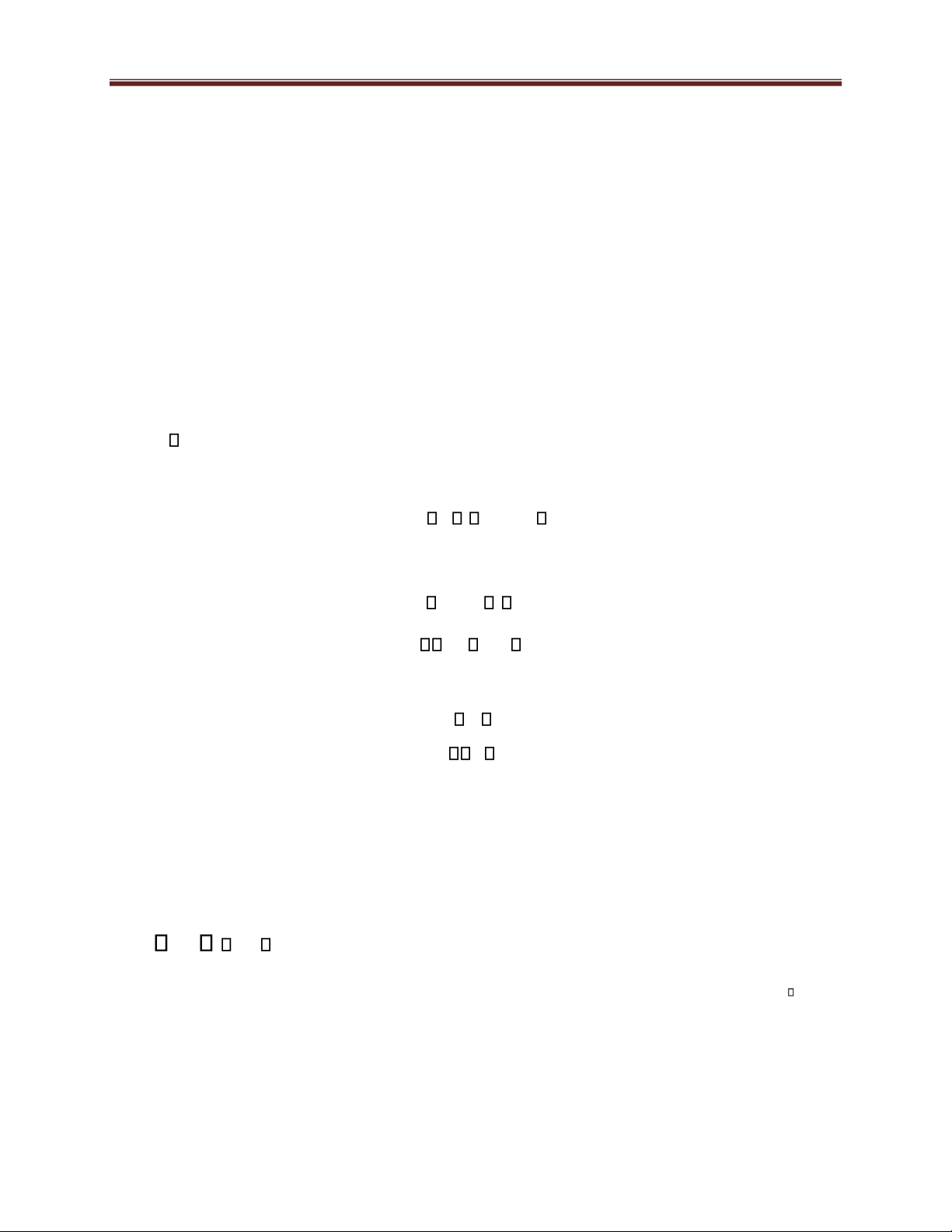
.x2 ... xin .xn bi (i = 1, 2, ..., n) x1 x2 xn Let a xik ik
(i, k = 1, 2, ..., n), then aik is the average of the costs that industry k xk 1 lOMoAR cPSD| 49519085
Lecturer: Nguyen Duong Nguyen, Mathematics Department, Faculty of Basic Science, FTU
must pay for the purchase of the product of industry i calculated for 1 unit of product
value of industry k. For example, a ik 0.4 means that in order to produce 1 unit of
product value, industry k has to buy 0.4 unit value of product of industry i on
average. It is easy to see that 0 aik 1.
We get the system of equations:
x1 a x11 1 + a12x2 + ... + a1nxn + b1
(1 a )x11 1 - a12x2 - ... - a1nxn = b1 x2 a x211 + a 22x2 + ... + a2nxn + b2
a x21 1 + (1-a22)x2 - ... - a2nxn = b2
..................................................
..................................................
xn a xn1 1 + an2x2 + ... + annxn + bn
a xn1 1 - an2x2 - ... + (1-ann)xn = bn a11 a ... a 12 1n x1 b 1 Put A a21 a22 ... a2n , X x2 , b b2 . ... ... ... an1 a n2 ... ann xn b m
A is called the input-coefficient matrix (the consumption matrix). X is called the total
demand matrix. b is called the final demand matrix.
We see that the sum of all the elements in column k of A is the cost that industry k
must pay for purchasing of factors of production to produce one unit of product value of industry k.
The above system of equations can be expressed in the form: (E - A) X = b. If E - A
is invertible, the total demand matrix is determined by the following formula: X E A 1 b. 2 lOMoAR cPSD| 49519085
Lecturer: Nguyen Duong Nguyen, Mathematics Department, Faculty of Basic Science, FTU
The matrix E – A is called the Leontief matrix.
Example. Suppose there are 3 industries in an economy: industry 1, industry 2,
industry 3. Let the input-coefficient matrix be: 0.4 0.1 0.2 0.3 A 0.2 0.4 0.2 0.1 0.3
with the final demand for products of each industry, respectively 40, 40 and 110
(unit: trillion VND). Determine the total demand for the products of each industry
and the total cost of the products used as production inputs for each industry.
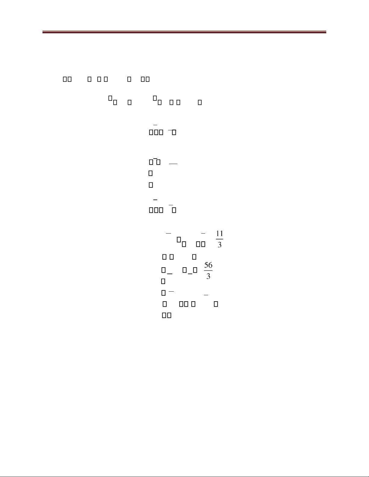
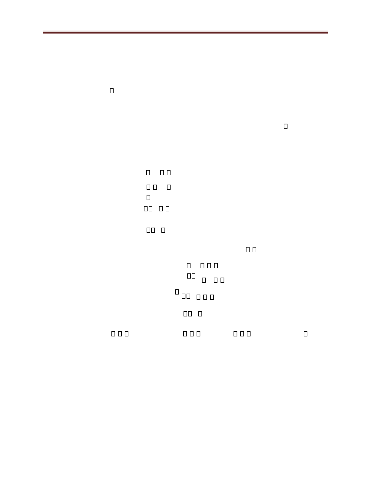
Solution. We have 1 0 0 0.4 0.1 0.2 0.6 0.1 0.2 E A 0 10 0.20.30.2 0.20.7 0.2 0 0 1 0.1 0.4 0.3 0.1 0.4 0.7 Then 2.05 0.75 0.8 (E A) 1 0.8 2 0.8 . 0.75 1.25 2
The total demand matrix is determined by . 0.8 40 x1 2.05 0.75 200 Therefore, the total X x2 0.8 2 0.8 . 40 demand for products 1.25 200 of industries 1, 2, 3 is x3 0.75 2 110 300 3 lOMoAR cPSD| 49519085
Lecturer: Nguyen Duong Nguyen, Mathematics Department, Faculty of Basic Science, FTU
respectively x1 = 200 trillion dong, x2 = 200 trillion dong and x3 = 300 trillion dong.
The total cost for the products used as production inputs for industry 1 is:
(0.4 + 0.2 + 0.1) .200 = 140 trillion dong.
The total cost for the products used as production inputs for industry 2 is:
(0.1 + 0.3 + 0.4) .200 = 160 trillion dong.
The total cost for the products used as production inputs for s industry 3 is:
(0.2 + 0.2 + 0.3) .300 = 210 trillion VND.
4.2. Market equilibrium model for n related commodities
Suppose we study a market consisting of n related commodities: commodity 1,
commodity 2,…, commodity n. This concept is understood that when the price of a
certain commodity changes, it not only affects the quantity supplied and quantity
demanded of that commodity, but also affects to the price and quantity supplied and
quantity demanded of the rest of commodities. To consider a market equilibrium
model for n related commodities, we symbol:
QSi : the quantity supplied supply of commodity i
QDi : the quantity demanded for commodity i Pi: the price of commodity i.
We express the dependence of the quantity supplied and quantity demanded on
the prices of commodities by the supply and demand functions as follows: QS S (P ,P ,..., P ) i i 1 2 n QD D (P ,P ,..., P ) i i 1 2 n i = 1, 2, 3, … , n 4 lOMoAR cPSD| 49519085
Lecturer: Nguyen Duong Nguyen, Mathematics Department, Faculty of Basic Science, FTU
The market equilibrium model for n related commodities: QSi QDi i 1,2,3,...,n
If the supply and demand functions are linear, the above model is a system of
linear equations consisting of n equations and n unknowns P1, P2, ..., Pn. Solving this
system of linear equations, we will find the equilibrium prices of all n commodities: P ,P , ...,P1 2 n
Substitute P ,P , ...,P1 2 n into supply functions (or demand functions), we get the
equilibrium quantity of each commodity: Q ,Q , ...,Q1 2 n
Example. Considering the market consisting of 3 commodities, including tea,
coffee, and cocoa, the supply and demand functions are as follows: QS 10 20 P 1 P ; Q1 D1 P1 3 (tea) QS 2P ; Q 40 2 2 D2 2P2 P3 (coffee) QS 5 10 P P 3 3P ; Q32 D3 P2 3 1 (cacao)
Determine the equilibrium price and the equilibrium quantity of above three commodities.
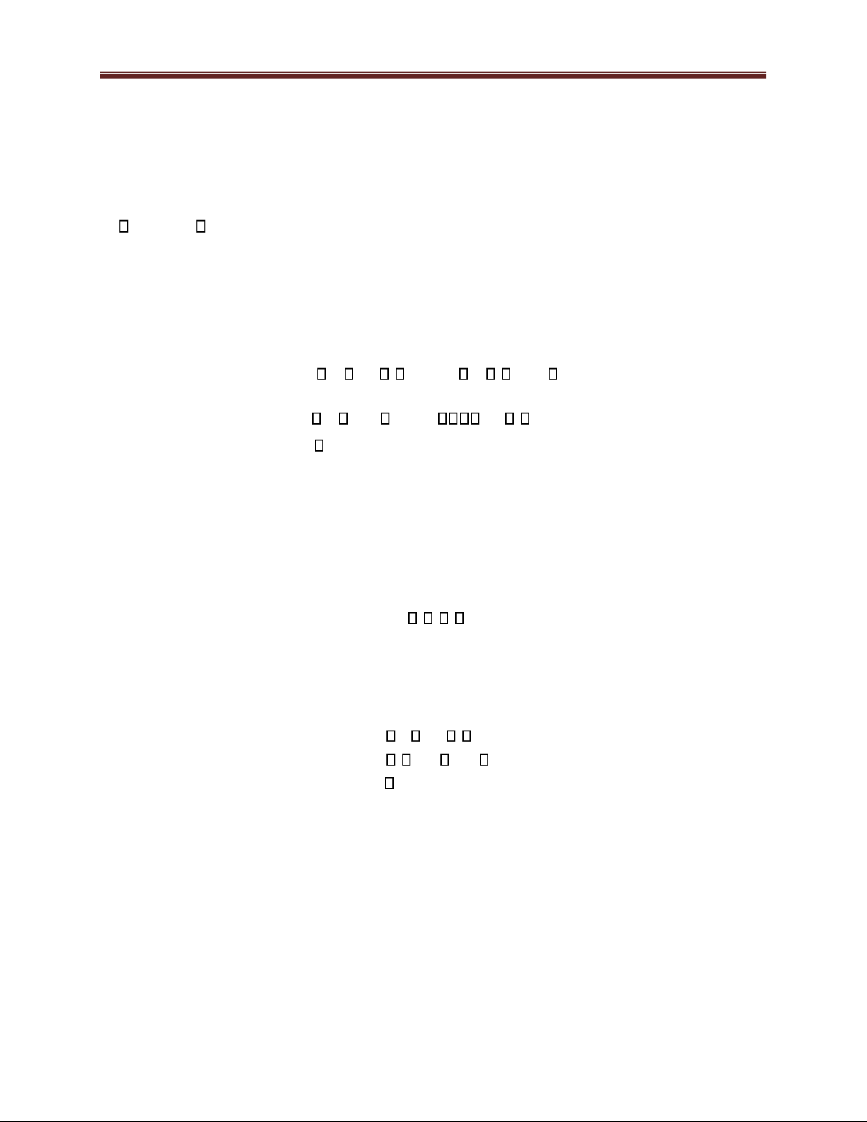
Solution. We establish the market equilibrium model for 3 related commodities: QS Q 2P P 30 1 D1 1 3 5 lOMoAR cPSD| 49519085
Lecturer: Nguyen Duong Nguyen, Mathematics Department, Faculty of Basic Science, FTU QS 2 D2 2 P3 40 Q 4P QS 3 QD3 P 1 P24P3 15 P1 413 28
The equilibrium prices are: P2 3 P3 83 Q1 10 P1 2
The equilibrium quantities are: Q 2P2 Q3 5 3P3 3
4.3. The national income equilibrium model
Consider the national income equilibrium model in simple form with the following symbols:
Y stands for the national income
G stands for the expenditure of the government
I stands for costs for investment by manufacturers
C stands for the consumption expenditure of households 6 lOMoAR cPSD| 49519085
Lecturer: Nguyen Duong Nguyen, Mathematics Department, Faculty of Basic Science, FTU
Here, we assume that the expenditure of the government and investment are fixed
G G0 andI I0 , while the consumption expenditure of households has a linear form:
C = aY + b (0 < a < 1; b > 0)
The national income equilibrium model has the form of a system of linear
equations with two equations and two unknowns Y and C: Y Go Io C Y C Go Io C AY b aY C b
Solving the above system, we determines the equilibrium national income and
the equilibrium consumption of the economy.
Next, consider the model in the case of taxable income with tax rate t (expressed
in decimal). Then, after-tax income is: Yd YtY (1 t)Y
and the consumption expenditure has the form: C = aYd + b = a(1 – t)Y + b. In
this case, we the national income equilibrium model is Y Go Io C
a(1 t Y) b C
For example. Let C = 0,80Yd + 250, I = Io, G = Go, Yd = (1- t)Y ( t is the income tax rate)
Determine the equilibrium national income and equilibrium consumption,
knowing that Io = 150 ; Go = 500 (unit: billion VND) and t = 0,15. 7 lOMoAR cPSD| 49519085
Lecturer: Nguyen Duong Nguyen, Mathematics Department, Faculty of Basic Science, FTU
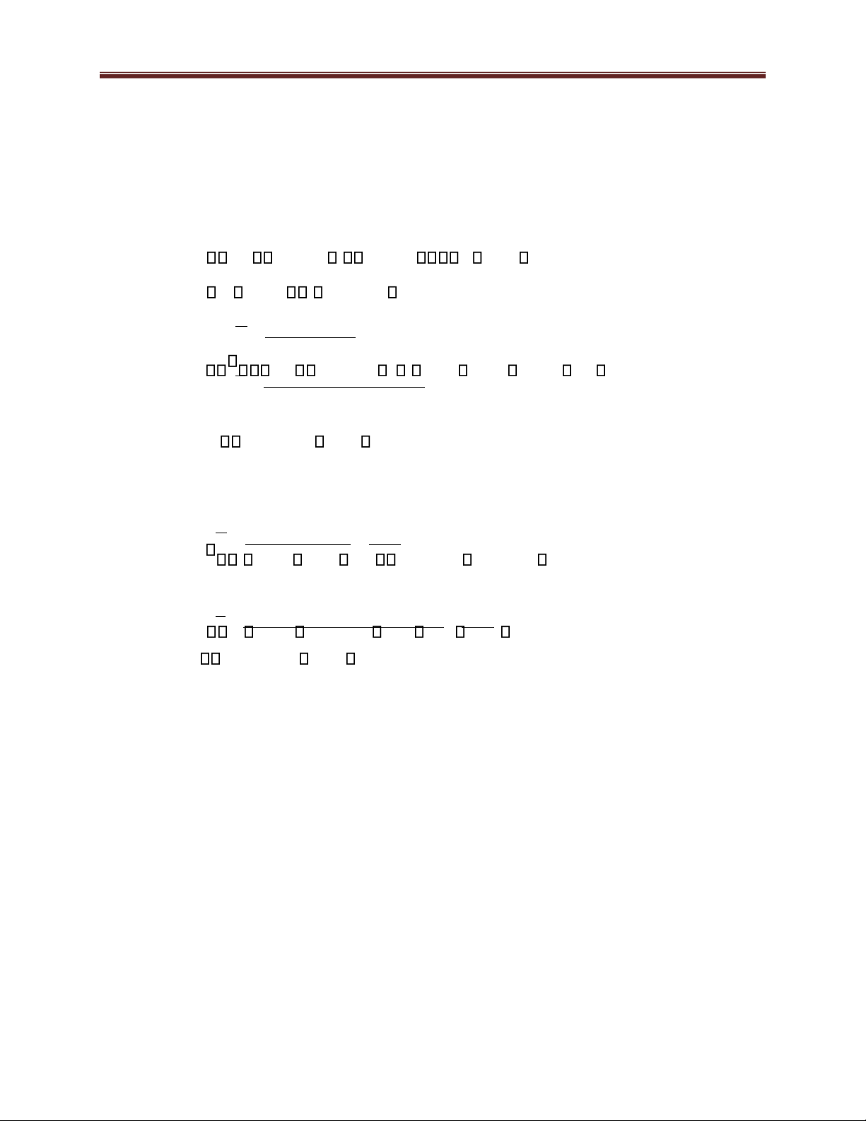
Solution. We get the national income equilibrium model CY 0G,8Yo Io250C Y 0,8(1 C Gt)Yo ICo 250 Y C
0,8(1G1 o 0,8(1 Iot)(G 250t)o I )o 250 1 0,8(1 t)
With Io = 150 ; Go = 500 ; t = 0,15, we have Y 1501 0,8(1 500
0,15)250 0900,32 2812,5 (billion VND)
C 0,8(1 0,15)(150 500) 250 692 2162,5 (billion VND) 1 0,8(1 0,1 )5 0,32 4.4. IS – LM model
Equilibrium in IS-LM model is characterized by an income level and interest rates
that simultaneously produce equilibrium in both the goods market and the money market.
Considering a goods market including the following elements: -
The government spending G = Go -
The consumption C = aY + b (0 < a < 1; b > 0) (or C = a(1-t)Y +b ; t is the taxes) 8 lOMoAR cPSD| 49519085
Lecturer: Nguyen Duong Nguyen, Mathematics Department, Faculty of Basic Science, FTU -
The investment I = k – lr (k, l > 0).
Denoted the level of gross domestic product (GDP) by Y.
A goods market is described by the following equation:
Y = C + I + Go = aY + b + k –lr +Go (1 –a)Y + lr = b + k + Go (1) (1) is called IS equation.
Considering the money market including the following elements:
- the money demand L = mY – nr (m, n > 0) - the money supply M = Mo.
The equilibrium condition of the money market is: L M mY nr Mo (2) (2) is called LM equation.
To determine the equilibrium national income level Y and the equilibrium interest
rates, we solve the following system of linear equations : (1 a)Y lr b k Go mY nrMo (3)
To solve this system, we can determine the equilibrium national income and equilibrium interest rate.
Example. Consider the model IS - LM with C = 0,6Y + 35 I = 65 – r Go = 70 (VND trillion) 9 lOMoAR cPSD| 49519085
Lecturer: Nguyen Duong Nguyen, Mathematics Department, Faculty of Basic Science, FTU L = 5Y – 50r Mo = 1500 (VND trillion)
Determine the equilibrium national income level and the equilibrium interest rate. Solution. Equation of the IS curve:
Y = C + I + Go = 0,6Y + 35 + 65 – r +70 0,4Y + r = 170 The equation of the LM curve:
L M o 5Y 50r 1500 Solve the system of equations 0,4Y r 170 5Y 50r 1500 We have Y 400 r 10 .
4.5. Optimization problem of two-variable linear function on convex polygon
domain in economics and business
Problem. Find the maximum and minimum value of the expression P x;y
ax by (a, b are two given numbers that are not simultaneously zero),
where x, y are the coordinates of points in the polygon domain A A ...A A1 2 i i 1 ...A .n
Determine x, y such that F reaches the maximum and minimum values. 10 lOMoAR cPSD| 49519085
Lecturer: Nguyen Duong Nguyen, Mathematics Department, Faculty of Basic Science, FTU
The above problem means: Let the expression P x;y ax by, and the convex
polygon domain (S) in the coordinate plane Oxy. Find the maximum and minimum
value of P x;y ax by, where (x;y) is the coordinate of point M in (S). Solution:
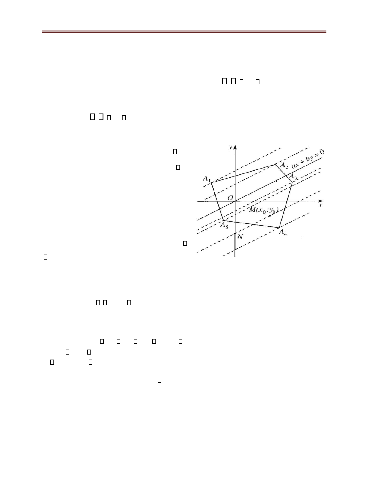
We illustrate the solution in the case n 5
and only consider the case b 0
(remaining cases are considered similar).
Assume that M(x ,y )0 0 is a given point
belongs to the polygon domain. Through
each point M and each vertex of the
polygon, draw lines parallel to the line ax by 0.
Among those lines, the line through the point M has the equation Figure 1 ax by ax0 by0
and intersects the vertical axis at point ax0 by0 0 , ax0 by0 is N 0; . Since b b ax0 by0 greatest if and only if is b 11 lOMoAR cPSD| 49519085
Lecturer: Nguyen Duong Nguyen, Mathematics Department, Faculty of Basic Science, FTU greatest.
In Figure 1, P = ax by is largest when (x;y) is the coordinate of point A1, smallest
when (x;y) is the coordinate of point A4 .
In summary, the maximum and minimum values of the expression P ax + by are
obtained at one of the vertices of the polygon domain.
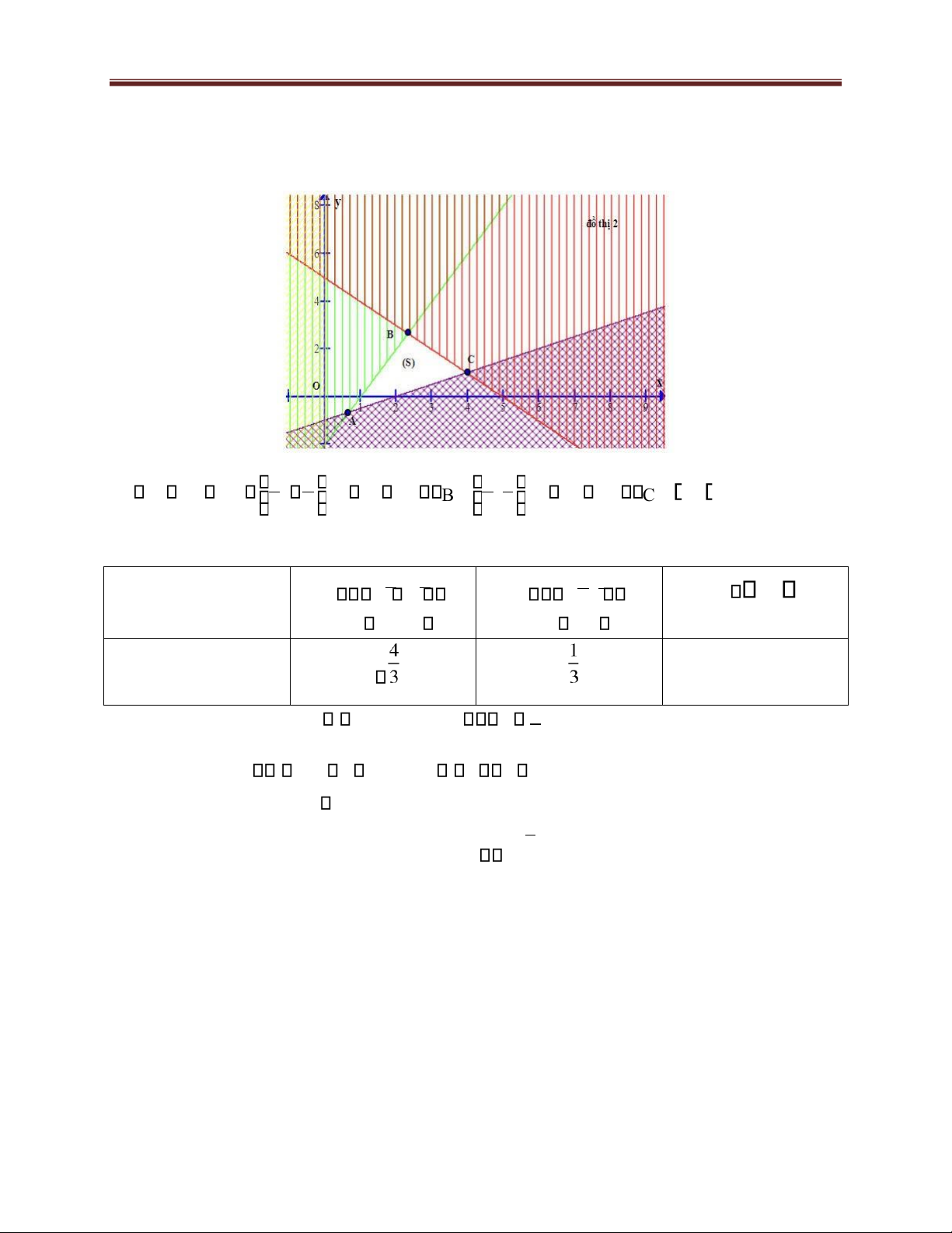
Example 1. Let x, y be real numbers satisfying the condition 2x y 2 2y 2 x x y 5 (1) x 0
Find the minimum and maximum value of the expression P y x. 2x y 2 0 x 2y 2 0
Solution. The system of equations (1) x y 5 0 x 0 Draw 4 lines d :2x1 y 20,d :x2 2y 20,d :x3 y 5 0,d :x4 0.
Crossing out the unsatisfactory half-planes, we get the solution domain (S) of system
(1) which is the triangle ABC (including the boundary). 12 lOMoAR cPSD| 49519085
Lecturer: Nguyen Duong Nguyen, Mathematics Department, Faculty of Basic Science, FTU 2 2 78 A 1 d d2 A ; ,B 1 d d3 B ; ,C d2 d3 C 4; 1 3 3 33
The table of values for P at the vertices of triangle ABC is Vertex A 2; 2 B 7 8; C 4;1 3 3 3 3 The value of P -3 4 1 x 73 Therefore, minP 3 x 1 , maxP 3 y 8 y 3
Example 2. In a bartending contest, each team can use up to 24g of flavoring, 9 liters
of water and 210g of sugar to make orange juice and apple juice. To prepare 1 liter
of orange juice requires 30g of sugar, 1 liter of water and lg of flavoring. To prepare
1 liter of apple juice requires 10g of sugar, 1 liter of water and 4g of flavoring. Each
liter of orange juice prepared will have 60 bonus points, and each liter of apple juice 13 lOMoAR cPSD| 49519085
Lecturer: Nguyen Duong Nguyen, Mathematics Department, Faculty of Basic Science, FTU
will get 80 bonus points. Ask how much you need to mix each type to get the highest score.
Solution. Let x and y be the number of liters of orange juice and apple juice to be prepared (x 0,y 0 )
- The number of bonus points obtained is P 60x 80y
- The number of liters of water used is x y 9
- The number of grams of sugar used is 30x 10y 210 or 3x y 21
- The number of grams of flavoring used is x 4y 24
According to the problem, we need to find the maximum value of P 60x 80y, where
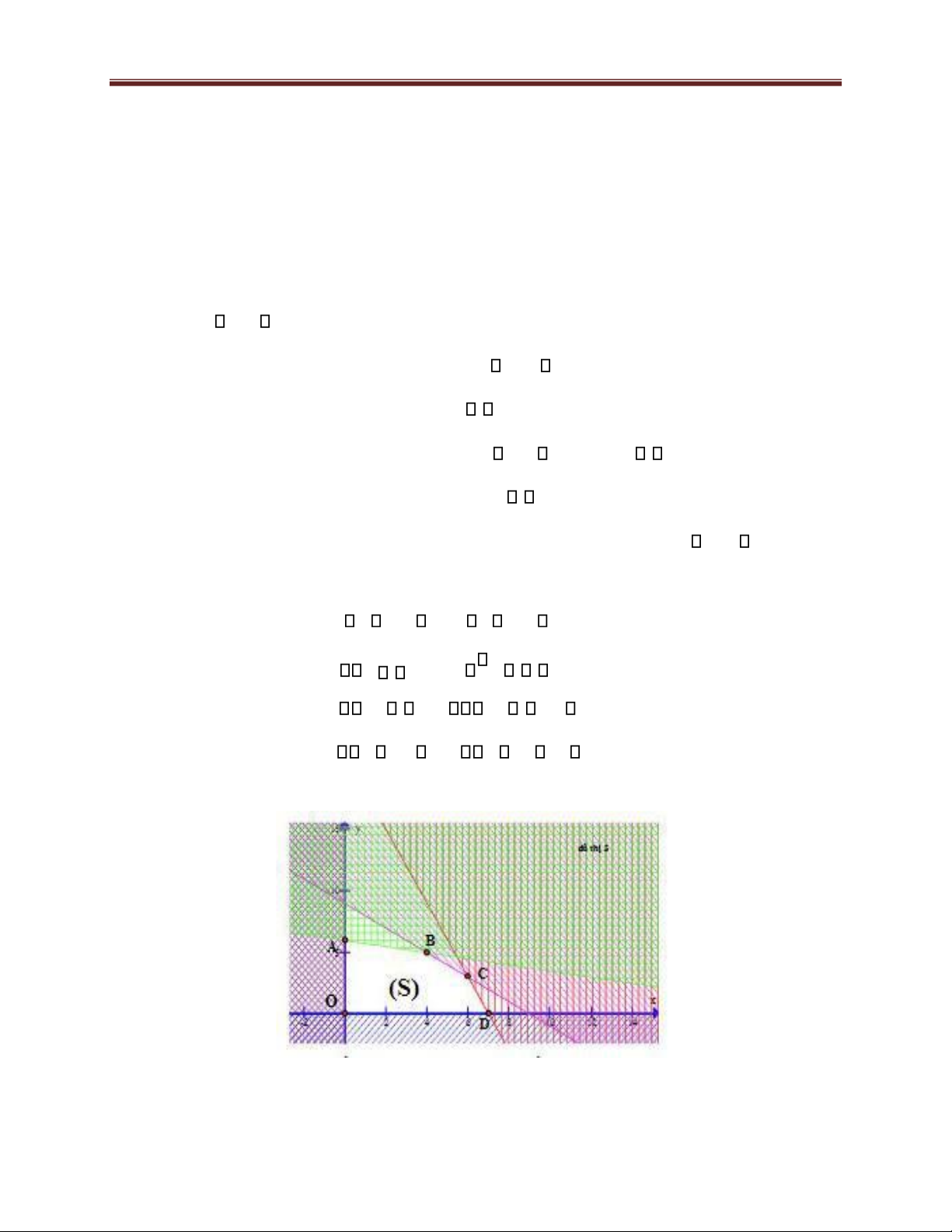
x, y are real numbers that satisfy x 0,y 0 x 0,y 0 x y9 x y9 0 3x y21 3x y 21 0 (2) x 4y 24 x 4y 24 0
The graph describing the solution domain of (2) is: 14 lOMoAR cPSD| 49519085
Lecturer: Nguyen Duong Nguyen, Mathematics Department, Faculty of Basic Science, FTU
From the graph, we have the solution domain (S) of system (2) which is the
pentagonal domain OABCD (including the boundary).
The coordinates of the vertices are O(0;0) , A(0;6), B(4;5) , C(6;3), D(7;0).
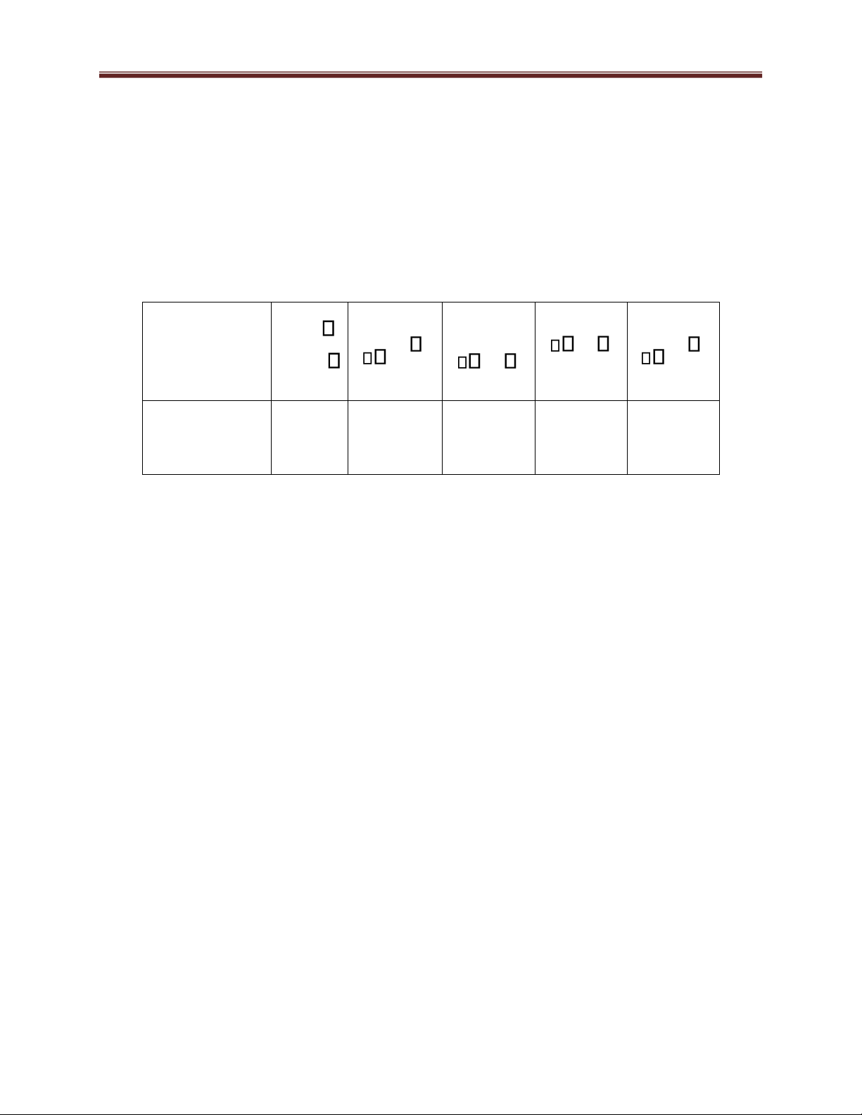
The calculation of the value of bonus points at the vertices is Vertex A C D O 0;0 B 6;3 0;6 4;5 7;0 Bonus points 0 480 640 600 280 P
So, the option with the highest bonus points is 4 liters of orange juice and 5 liters of apple juice. 15