









Silde bài giảng chương 5 môn toán cao cấp ( Tiếng anh chất lượng cao )

Partial differentiation: a technique for deriving the rate of change of a function w/respect to increase an independence variable while other independence variables are held constant.  For example: if the production function Q=f(K,L) is differentiated with respect to L, K held constant=> getting rate of change of total product with respect to L (in other words: MPL). Tài liệu giúp bạn tham khảo, ôn tập và đạt kết quả cao. Mời bạn đọc đón xem !

Môn:
Thông tin:
21 trang 2 tháng trước

Bình luận

Vui lòng đăng nhập hoặc đăng ký để gửi bình luận.

Silde bài giảng chương 5 môn toán cao cấp ( Tiếng anh chất lượng cao )

Partial differentiation: a technique for deriving the rate of change of a function w/respect to increase an independence variable while other independence variables are held constant.  For example: if the production function Q=f(K,L) is differentiated with respect to L, K held constant=> getting rate of change of total product with respect to L (in other words: MPL). Tài liệu giúp bạn tham khảo, ôn tập và đạt kết quả cao. Mời bạn đọc đón xem !

39 20 lượt tải Tải xuống
CONTENT
Partial differentiation and the
1 marginal product
Second-order partial derivatives
2
Unconstrained optimization: function 3 with two
variables
Total differentials and total
lOMoARcPSD| 46578282
7/29/2020
1
CHAPTER 5: PARTIAL
DIFFERENTIATION
PREPARED BY: FINANCE DEPARTMENT
COURSE CODE:
B03013
B03013 – Chapter 5: Partial
7/29/2020 1
differentiation
7/29/2020
B03013 – Chapter 5: Partial differentiation
2
LEARNING OBJECTIVES
the
partial
differentiation
and
applications
Introduce
the
second
order
partial
derivatives
The forms
of total differentials and total
derivatives
lOMoARcPSD| 46578282
7/29/2020
2
4 derivatives
7/29/2020
B03013 – Chapter 5: Partial differentiation
3
Partial and total differentiation.
Unconstrained optimization.
Partial and total differentiation.
7/29/2020
B03013 – Chapter 5: Partial differentiation
4
CONCEPTS
lOMoARcPSD| 46578282
7/29/2020
3
Y= 14x+ 3z
2
Y= 6x
2
z
7/29/2020
B03013 – Chapter 5: Partial differentiation
5
Partial differentiation and the
marginal product
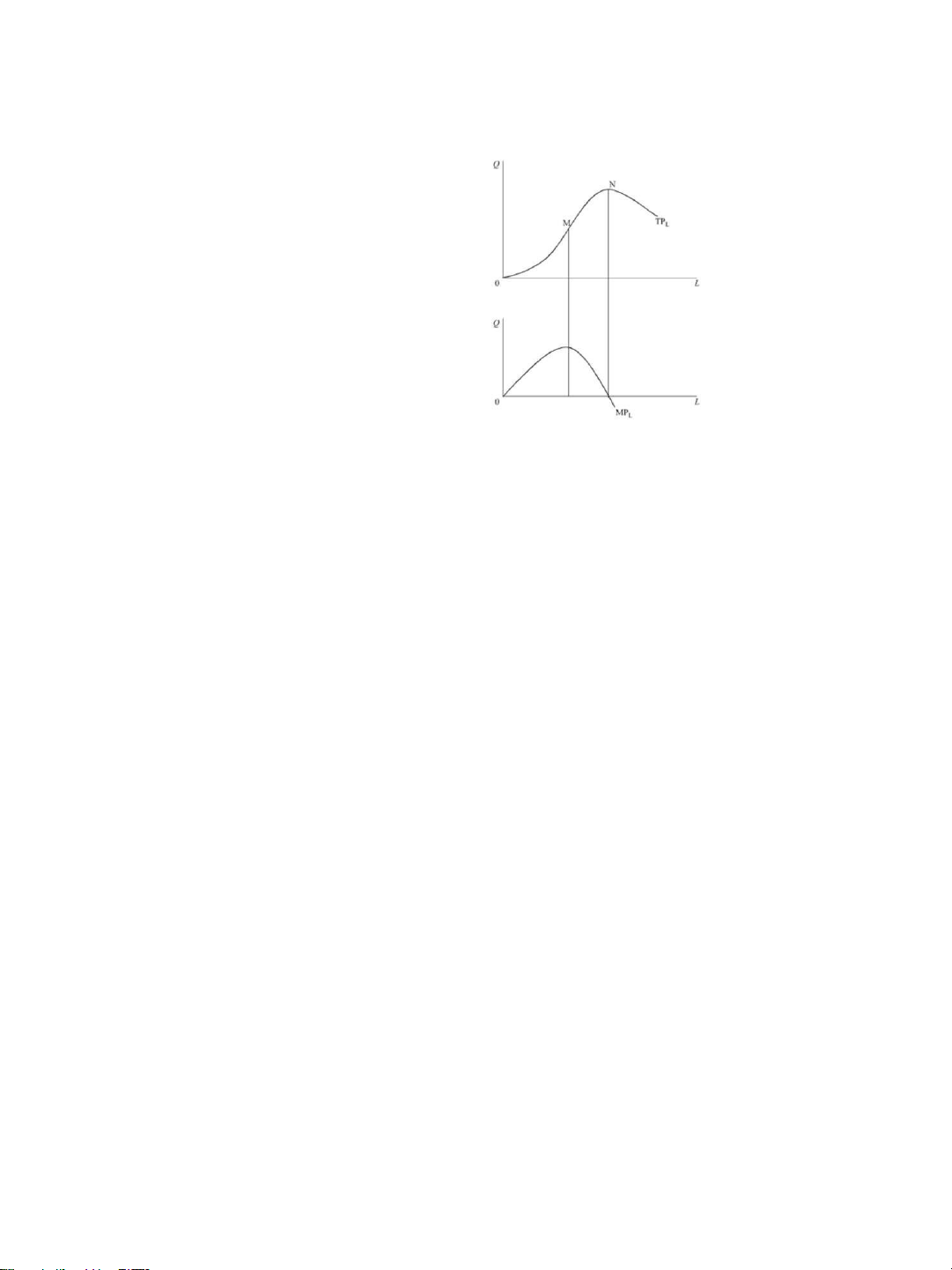
Partial differentiation: a technique for deriving
the rate of change of a function w/respect to
increase an independence variable while other
independence variables are held constant.
For example: if the production function Q=f(K,L)
is differentiated with respect to L, K held
constant=> getting rate of change of total
product with respect to L (in other words: MP
L
).
7/29/2020
B03013 – Chapter 5: Partial differentiation
6
lOMoARcPSD| 46578282
7/29/2020
4
MP
L
lOMoARcPSD| 46578282
7/29/2020
5
Basic rule: all independent variables, other than
the one that the function is being differentiated with
respect, are treated as constant. ( Q/ L)
7/29/2020
B03013 – Chapter 5: Partial differentiation
7
Partial differentiation and the
marginal product
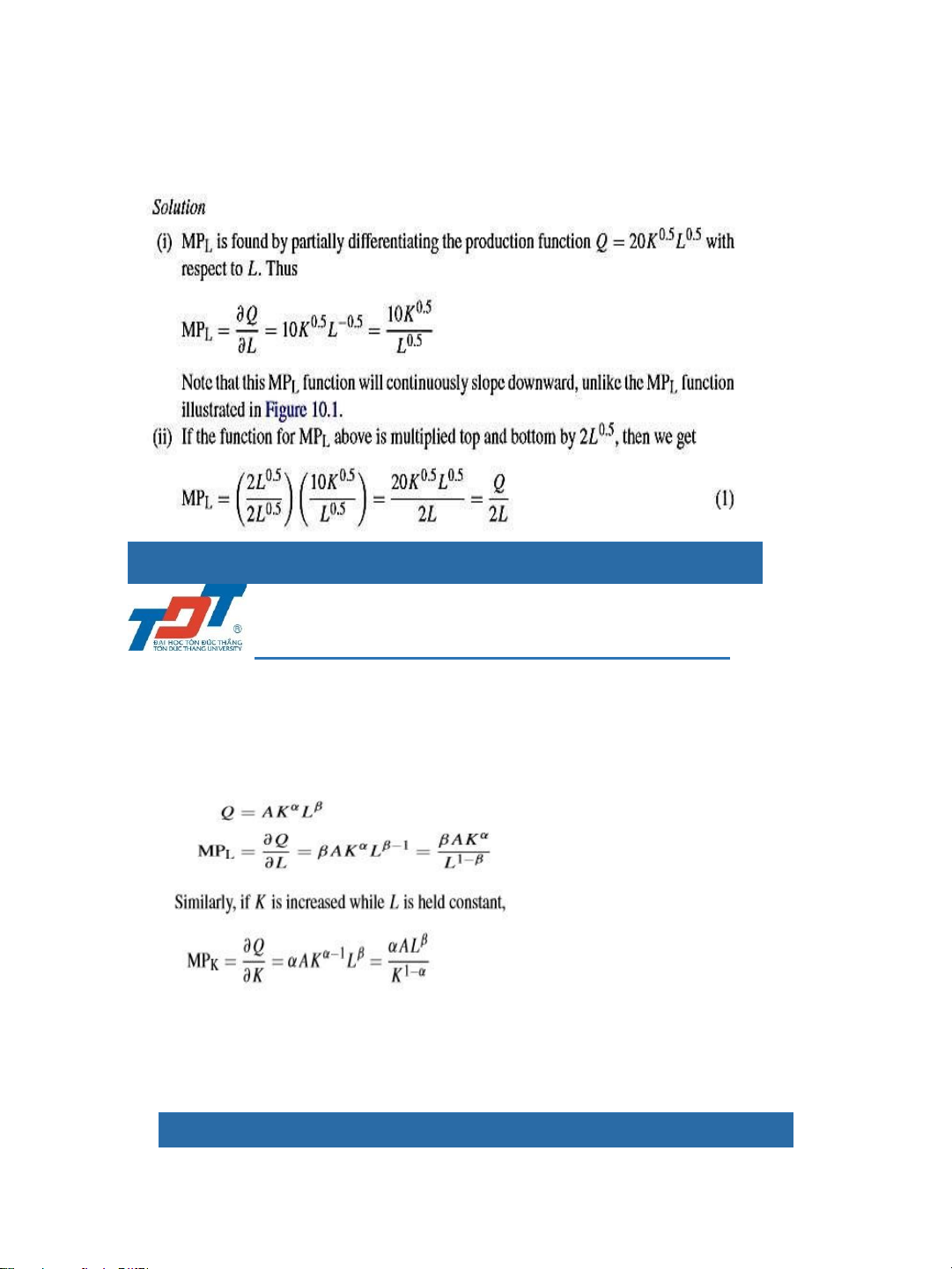
Example: For the production function
Q=20K0.5L0.5
1. Derive a function for MP
L
.
2. Show that MP
L
decreases as one moves along
an isoquant by using more L.
Other examples in [1] P.290-296
7/29/2020
B03013 – Chapter 5: Partial differentiation
8
lOMoARcPSD| 46578282
7/29/2020
6
Example
7/29/2020
B03013 – Chapter 5: Partial differentiation
9
A Cobb- Douglas Production Function
Q= AK
α
L
β
If K is held constant then
Example
Q=20K0.4L0.5
7/29/2020
B03013 – Chapter 5: Partial differentiation
10
Marginal product
lOMoARcPSD| 46578282
7/29/2020
7
Q= 4.6K
2
+ 3.5L
2
- 0.012K
3
L
3
q=
20x0.6y00.2z0.3
7/29/2020
B03013 – Chapter 5: Partial differentiation
11
Further application
Elasticity: in a market, the quantity demanded,
q, depends on several factors (price: p,
average income: m, price of a
complement/substitute: p
c
/p
s
; and the
population: n).
Price elasticity of demand is usually defined as:
e=(-1)(percentage change in quantity
demanded)/(percentage change in price).
7/29/2020
B03013 – Chapter 5: Partial differentiation
12
lOMoARcPSD| 46578282
7/29/2020
8
Ceteris paribus: assume other factors/vars
held constant.
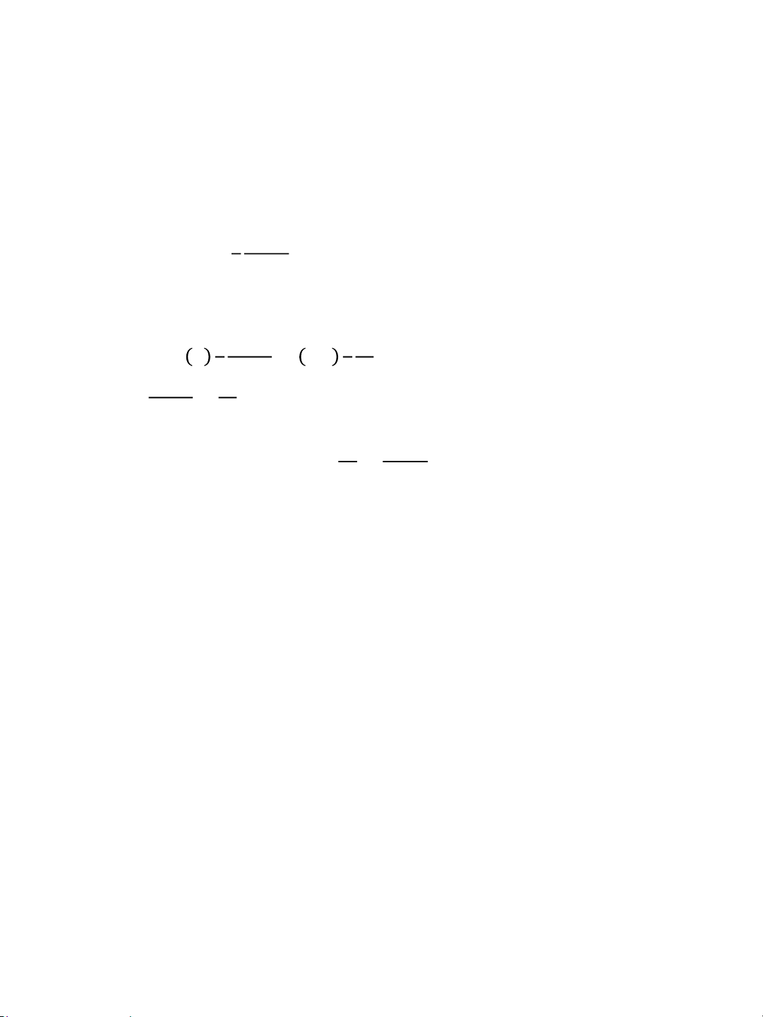
𝑒 = (1)
𝑝 1
;
𝑞𝑑𝑝 𝑑𝑞
recognizing that quantity demanded depends on
factors other than price, then
𝑒 = 1
𝑝 1
= −1
𝑝𝜕𝑞
𝑞𝜕𝑝 𝜕𝑞 𝑞𝜕𝑝
1
=
𝜕𝑞
from an inverse function (for
𝜕𝑝 𝜕𝑞 𝜕𝑝
example, y=f(x) then
𝑑𝑥
=
1
)
𝑑𝑦 𝑑𝑦 𝑑𝑥
lOMoARcPSD| 46578282
7/29/2020
9
7/29/2020
B03013 – Chapter 5: Partial differentiation
13
Other measures of elasticity: depending n other
variables, for example:
e
m
=(percentage change in quantity
demanded)/(percentage change in income).
∆𝑞
𝑒𝑚 = 𝑚𝑞 = 𝑚𝑞 ∆𝑚∆𝑞 = 𝑚𝑞 𝜕𝑚𝜕𝑞
𝑚
Consumer utility functions: U=U(x
1
,x
2
,…,x
n
)
where x
1
, x
2
,…,x
n
: amount of the different good
consumed.
If we assume two goods A and B are consumed,
then U=U(A,B).
7/29/2020
B03013 – Chapter 5: Partial differentiation
14
Further application
lOMoARcPSD| 46578282
7/29/2020
10
=> Marginal utility: rate of change of total utility with
respect to the increase in consumption of one
goods, therefore 𝑀𝑈
𝐴
=
𝜕𝑈
𝜕𝐴
𝑎𝑛𝑑𝑀𝑈
𝐵
=
𝜕𝑈
𝜕𝐵
7/29/2020
B03013 – Chapter 5: Partial differentiation
15
3 important principles of utility theory:
(i). The law of diminishing marginal say: if, ceteris
paribus, the quantity consumed of any one good is
increased, then eventually, its marginal utility will
decline.
(ii). A consumer will consume a good up to the point
where its MU=0 if it is a free good, or if a fixed
payment is made regardless of the quantity
consumed (water rates).
(iii). A consumer maximizes satisfaction when
each good is consumed up to the point where
an extra unit spent on one good will derive the
same utility as an extra unit spent on any other
good.
Other applications: Keynesian multiplier, cost
and revenue function
7/29/2020
B03013 – Chapter 5: Partial differentiation
16
Further application
lOMoARcPSD| 46578282
7/29/2020
11
7/29/2020
B03013 – Chapter 5: Partial differentiation
17
Second order partial derivatives
Being found by differentiating the first-order
partial derivatives of a function.
If a function has two independent variables, there
will be four second-order partial derivatives. For a
fn y=f(x,z)
(i) 𝜕𝜕𝑥2𝑦2 (ii) 𝜕𝜕𝑧2𝑦2 (iii) 𝜕𝑥𝜕𝑧𝜕2𝑦
(iv) 𝜕𝑧𝜕𝑥𝜕2𝑦
while (iii) and (iv) are equal
Example: derive Q=6K+0.3K
2
L+1.2L
2
and
interpret their meaning.
7/29/2020
B03013 – Chapter 5: Partial differentiation
18
lOMoARcPSD| 46578282
7/29/2020
12
Unconstrained optimization
If we have two variable fn y=f(x,z) to be at a
maximum or at a minimum, the 1
st
-order
conditions which must be met are:
𝜕𝑦
= 0 and
𝜕𝑦
= 0
𝜕𝑥 𝜕𝑧
lOMoARcPSD| 46578282
7/29/2020
13
To be at a max or min, the function must be at
a stationary point with respect to changes in
both variables. The 2
nd
-order conditions for the
optimization of multivariable functions with a fn
y=f(x,z)
7/29/2020
B03013 – Chapter 5: Partial differentiation
19
Unconstrained optimization
𝜕
𝜕𝑥
2
𝑦
2
< 0 and
𝜕
𝜕𝑧
2
𝑦
2
<0 for a minimum
𝜕
2
𝑦
2
>0 and
𝜕
𝜕𝑧
2
𝑦
2
>0 for a maximum
𝜕𝑥
And the other 2
nd
-order condition:
𝜕𝜕𝑥2𝑦2 𝜕𝜕𝑧2𝑦2 > 𝜕𝑥𝜕𝑧𝜕2𝑦 2
Example 1
A firm produces two products which are sold in
two separate markets with the demand
schedules
p1= 600-0.3q1 p2= 500-0.2q2
Production costs are related and the firm faces
the total cost function
TC= 16+1.2q1+1.5q2+0.2q1q2
7/29/2020
B03013 – Chapter 5: Partial differentiation
20
lOMoARcPSD| 46578282
7/29/2020
14
If the firm wishes to maximize total profits, how
much of each product should it sell? What will
the maximum profit level be?
7/29/2020
B03013 – Chapter 5: Partial differentiation
21
A multiplant monopoly operates two plants
whose total cost schedules are
TC1= 8.5 +0.03q
1
2
TC2=5.2+0.04q
2
2
If it
faces the demand schedule p= 60-0.04q
Where q= q1+q2, how much should it produce
in each plant in order to maximize profit?
7/29/2020
B03013 – Chapter 5: Partial differentiation
22
Example 2
lOMoARcPSD| 46578282
7/29/2020
15
Unconstrained optimization
lOMoARcPSD| 46578282
7/29/2020
16
Exercise 1: a firm operates with the production
function: Q=95K
0.3
L
0.2
R
0.25
and buys the three
inputs K, L and R at prices of $30, $16 and $12
per unit respectively. If it can sell its output at a
fixed price of $4 per unit, what is the maximum
profit it can make?
7/29/2020
B03013 – Chapter 5: Partial differentiation
23
Unconstrained optimization
Exercise 2: A multiplant monopoly has 2 plants
with whose total costs: TC
1
=36+0.003q
1
3
and
TC
2
=45+0.005q
2
3
if its total output is sold in a
market where demand: p=320-0.1q (q=q
1
+q
2
),
how much should it produce in each plant to
maximize its profit?
Total differentials and total
derivatives
If a non-linear fn y=f(x), the value dy/dx will
alter if x and y alter, it is therefore not possible
to predict the effect of a given increase in x on
y with complete accuracy. A very small
change ( x) in x => ∆𝑦 =
𝑑𝑦
∆𝑥
𝑑𝑥
(approximately true). If we have y=f(x,z)
then ∆𝑦 =
𝑑𝑦
∆𝑥 +
𝑑𝑦
∆𝑧 𝑑𝑥 𝑑𝑧
7/29/2020
B03013 – Chapter 5: Partial differentiation
24
lOMoARcPSD| 46578282
7/29/2020
17
Total differential. it can be write:
d𝑦 =
𝜕𝑦
𝑑𝑥 +
𝜕𝑦
𝑑𝑧
𝜕𝑥 𝜕𝑧
lOMoARcPSD| 46578282
7/29/2020
18
7/29/2020
B03013 – Chapter 5: Partial differentiation
25
Total differentials and total
derivatives
Total derivatives: in a production function the
amount of one input used may affect the
amount of another input that can be used with
it. From the total differential of a function we
can derive a total derivative which can cope
with this effect.
Assume y=f(x, z), and also x=g(z) => any
change in z will affect y as:
+ directly via the function f(x, z) and
+ indirectly by changing x via the function g(z),
which in turn will affect y via the function f(x, z).
Total differentials and total
derivatives
The total differential of y=f(x, z) is
𝑑𝑦 =
𝜕𝑦
𝑑𝑥 +
𝜕𝑦
𝑑𝑧 dividing through dz gives
𝜕𝑥 𝜕𝑧
𝑑𝑦
=
𝜕𝑦𝑑𝑥
+
𝜕𝑦
the 1st term: indirect effect of z-
𝑑𝑧 𝜕𝑥𝑑𝑧 𝜕𝑧
via its impact on x; and the 2
nd
term shows the
direct effect.
7/29/2020
B03013 – Chapter 5: Partial differentiation
26
| 1/21

Preview text:

CONTENT Partial differentiation and the 1 marginal product
Second-order partial derivatives 2
Unconstrained optimization: function 3 with two variables Total differentials and total lOMoAR cPSD| 46578282 7/29/2020 CHAPTER 5: PARTIAL DIFFERENTIATION
PREPARED BY: FINANCE DEPARTMENT COURSE CODE: B03013
B03013 – Chapter 5: Partial 7/29/2020 1 differentiation LEARNING OBJECTIVES
Define the partial differentiation and applications
Introduce the second order partial derivatives
The forms of total differentials and total derivatives 7/29/2020
B03013 – Chapter 5: Partial differentiation 2 1 lOMoAR cPSD| 46578282 7/29/2020 4 derivatives 7/29/2020
B03013 – Chapter 5: Partial differentiation 3 CONCEPTS
• Partial and total differentiation.
• Unconstrained optimization.
Partial and total differentiation. 7/29/2020
B03013 – Chapter 5: Partial differentiation 4 2 lOMoAR cPSD| 46578282 7/29/2020 • Y= 14x+ 3z2 • Y= 6x2z 7/29/2020
B03013 – Chapter 5: Partial differentiation 5
Partial differentiation and the marginal product
Partial differentiation: a technique for deriving
the rate of change of a function w/respect to
increase an independence variable while other
independence variables are held constant.
• For example: if the production function Q=f(K,L)
is differentiated with respect to L, K held
constant=> getting rate of change of total
product with respect to L (in other words: MPL). 7/29/2020
B03013 – Chapter 5: Partial differentiation 6 3 lOMoAR cPSD| 46578282 7/29/2020 MPL 4 lOMoAR cPSD| 46578282 7/29/2020
Basic rule: all independent variables, other than
the one that the function is being differentiated with
respect, are treated as constant. ( Q/ L) 7/29/2020
B03013 – Chapter 5: Partial differentiation 7
Partial differentiation and the marginal product
Example: For the production function Q=20K0.5L0.5 1. Derive a function for MPL.
2. Show that MPL decreases as one moves along an isoquant by using more L.
Other examples in [1] P.290-296 7/29/2020
B03013 – Chapter 5: Partial differentiation 8 5 lOMoAR cPSD| 46578282 7/29/2020 Example 7/29/2020
B03013 – Chapter 5: Partial differentiation 9 Marginal product
• A Cobb- Douglas Production Function Q= AKαLβ
• If K is held constant then Example • Q=20K0.4L0.5 7/29/2020
B03013 – Chapter 5: Partial differentiation 10 6 lOMoAR cPSD| 46578282 7/29/2020
• Q= 4.6K2+ 3.5L2 - 0.012K3L3 • q= 20x0.6y00.2z0.3 7/29/2020
B03013 – Chapter 5: Partial differentiation 11 Further application
Elasticity: in a market, the quantity demanded,
q, depends on several factors (price: p,
average income: m, price of a
complement/substitute: pc/ps; and the population: n).
• Price elasticity of demand is usually defined as:
• e=(-1)(percentage change in quantity
demanded)/(percentage change in price). 7/29/2020
B03013 – Chapter 5: Partial differentiation 12 7 lOMoAR cPSD| 46578282 7/29/2020
Ceteris paribus: assume other factors/vars held constant. • 𝑒 = (1) 𝑝 1 ; 𝑞𝑑𝑝 𝑑𝑞
• recognizing that quantity demanded depends on
factors other than price, then • 𝑒 = 1 𝑝 1 = −1 𝑝𝜕𝑞 𝑞𝜕𝑝 𝜕𝑞 𝑞𝜕𝑝
• 1 = 𝜕𝑞 from an inverse function (for 𝜕𝑝 𝜕𝑞 𝜕𝑝
example, y=f(x) then 𝑑𝑥 = 1 ) 𝑑𝑦 𝑑𝑦 𝑑𝑥 8 lOMoAR cPSD| 46578282 7/29/2020 7/29/2020
B03013 – Chapter 5: Partial differentiation 13 Further application
• Other measures of elasticity: depending n other variables, for example:
• em=(percentage change in quantity
demanded)/(percentage change in income). ∆𝑞
• 𝑒𝑚 = ∆𝑚𝑞 = 𝑚𝑞 ∆𝑚∆𝑞 = 𝑚𝑞 𝜕𝑚𝜕𝑞 𝑚
• Consumer utility functions: U=U(x1,x2,…,xn)
where x1, x2,…,xn: amount of the different good consumed.
• If we assume two goods A and B are consumed, then U=U(A,B). 7/29/2020
B03013 – Chapter 5: Partial differentiation 14 9 lOMoAR cPSD| 46578282 7/29/2020
=> Marginal utility: rate of change of total utility with
respect to the increase in consumption of one
goods, therefore 𝑀𝑈𝐴 = 𝜕𝑈𝜕𝐴 𝑎𝑛𝑑𝑀𝑈𝐵 = 𝜕𝑈𝜕𝐵 7/29/2020
B03013 – Chapter 5: Partial differentiation 15 Further application
• 3 important principles of utility theory:
(i). The law of diminishing marginal say: if, ceteris
paribus, the quantity consumed of any one good is
increased, then eventually, its marginal utility will decline.
(ii). A consumer will consume a good up to the point
where its MU=0 if it is a free good, or if a fixed
payment is made regardless of the quantity consumed (water rates).
• (iii). A consumer maximizes satisfaction when
each good is consumed up to the point where
an extra unit spent on one good will derive the
same utility as an extra unit spent on any other good.
• Other applications: Keynesian multiplier, cost and revenue function 7/29/2020
B03013 – Chapter 5: Partial differentiation 16 10 lOMoAR cPSD| 46578282 7/29/2020 7/29/2020
B03013 – Chapter 5: Partial differentiation 17
Second order partial derivatives
• Being found by differentiating the first-order
partial derivatives of a function.
• If a function has two independent variables, there
will be four second-order partial derivatives. For a fn y=f(x,z) • (i) 𝜕𝜕𝑥2𝑦2 (ii) 𝜕𝜕𝑧2𝑦2 (iii) 𝜕𝑥𝜕𝑧𝜕2𝑦 (iv) 𝜕𝑧𝜕𝑥𝜕2𝑦
• while (iii) and (iv) are equal
• Example: derive Q=6K+0.3K2L+1.2L2 and interpret their meaning. 7/29/2020
B03013 – Chapter 5: Partial differentiation 18 11 lOMoAR cPSD| 46578282 7/29/2020
Unconstrained optimization
• If we have two variable fn y=f(x,z) to be at a
maximum or at a minimum, the 1st-order
conditions which must be met are:
• 𝜕𝑦 = 0 and 𝜕𝑦 = 0 𝜕𝑥 𝜕𝑧 12 lOMoAR cPSD| 46578282 7/29/2020
• To be at a max or min, the function must be at
a stationary point with respect to changes in
both variables. The 2nd-order conditions for the
optimization of multivariable functions with a fn y=f(x,z) 7/29/2020
B03013 – Chapter 5: Partial differentiation 19
Unconstrained optimization
• 𝜕𝜕𝑥2𝑦2 < 0 and 𝜕𝜕𝑧2𝑦2<0 for a minimum
• 𝜕2𝑦2 >0 and 𝜕𝜕𝑧2𝑦2>0 for a maximum 𝜕𝑥
• And the other 2nd-order condition:
• 𝜕𝜕𝑥2𝑦2 𝜕𝜕𝑧2𝑦2 > 𝜕𝑥𝜕𝑧𝜕2𝑦 2 Example 1
A firm produces two products which are sold in
two separate markets with the demand schedules p1= 600-0.3q1 p2= 500-0.2q2
Production costs are related and the firm faces the total cost function TC= 16+1.2q1+1.5q2+0.2q1q2 7/29/2020
B03013 – Chapter 5: Partial differentiation 20 13 lOMoAR cPSD| 46578282 7/29/2020
If the firm wishes to maximize total profits, how
much of each product should it sell? What will the maximum profit level be? 7/29/2020
B03013 – Chapter 5: Partial differentiation 21 Example 2
• A multiplant monopoly operates two plants
whose total cost schedules are • TC1= 8.5 +0.03q 2 2 1 TC2=5.2+0.04q2 • If it
faces the demand schedule p= 60-0.04q
• Where q= q1+q2, how much should it produce
in each plant in order to maximize profit? 7/29/2020
B03013 – Chapter 5: Partial differentiation 22 14 lOMoAR cPSD| 46578282 7/29/2020
Unconstrained optimization 15 lOMoAR cPSD| 46578282 7/29/2020
Exercise 1: a firm operates with the production
function: Q=95K0.3L0.2R0.25 and buys the three
inputs K, L and R at prices of $30, $16 and $12
per unit respectively. If it can sell its output at a
fixed price of $4 per unit, what is the maximum profit it can make? 7/29/2020
B03013 – Chapter 5: Partial differentiation 23
Unconstrained optimization
Exercise 2: A multiplant monopoly has 2 plants with whose total costs: TC 3 1=36+0.003q1 and TC 3
2=45+0.005q2 if its total output is sold in a
market where demand: p=320-0.1q (q=q1+q2),
how much should it produce in each plant to maximize its profit?
Total differentials and total derivatives
• If a non-linear fn y=f(x), the value dy/dx will
alter if x and y alter, it is therefore not possible
to predict the effect of a given increase in x on
y with complete accuracy. • A very small
change ( x) in x => ∆𝑦 = 𝑑𝑦 ∆𝑥 𝑑𝑥
(approximately true). • If we have y=f(x,z)
then ∆𝑦 = 𝑑𝑦 ∆𝑥 + 𝑑𝑦 ∆𝑧 𝑑𝑥 𝑑𝑧 7/29/2020
B03013 – Chapter 5: Partial differentiation 24 16 lOMoAR cPSD| 46578282 7/29/2020
Total differential. it can be write:
d𝑦 = 𝜕𝑦 𝑑𝑥 + 𝜕𝑦 𝑑𝑧 𝜕𝑥 𝜕𝑧 17 lOMoAR cPSD| 46578282 7/29/2020 7/29/2020
B03013 – Chapter 5: Partial differentiation 25
Total differentials and total derivatives
Total derivatives: in a production function the
amount of one input used may affect the
amount of another input that can be used with
it. From the total differential of a function we
can derive a total derivative which can cope with this effect.
• Assume y=f(x, z), and also x=g(z) => any change in z will affect y as:
+ directly via the function f(x, z) and
+ indirectly by changing x via the function g(z),
which in turn will affect y via the function f(x, z).
Total differentials and total derivatives
The total differential of y=f(x, z) is
• 𝑑𝑦 = 𝜕𝑦 𝑑𝑥 + 𝜕𝑦 𝑑𝑧 dividing through dz gives 𝜕𝑥 𝜕𝑧
• 𝑑𝑦 = 𝜕𝑦𝑑𝑥 + 𝜕𝑦 the 1st term: indirect effect of z- 𝑑𝑧 𝜕𝑥𝑑𝑧 𝜕𝑧
via its impact on x; and the 2nd term shows the direct effect. 7/29/2020
B03013 – Chapter 5: Partial differentiation 26 18